[R] Fetching JSON: Data on the "GitHub to GitLab" Exodus from June 2018
Update: Further Reading included
1 The Setting
When news broke that Microsoft acquired GitHub on June 3rd 2018, Twitter was lit. I stumbled upon a Tweet with a link to GitLab’s dashboard where you could see various metrics for GitLab’s importer API for GitHub:
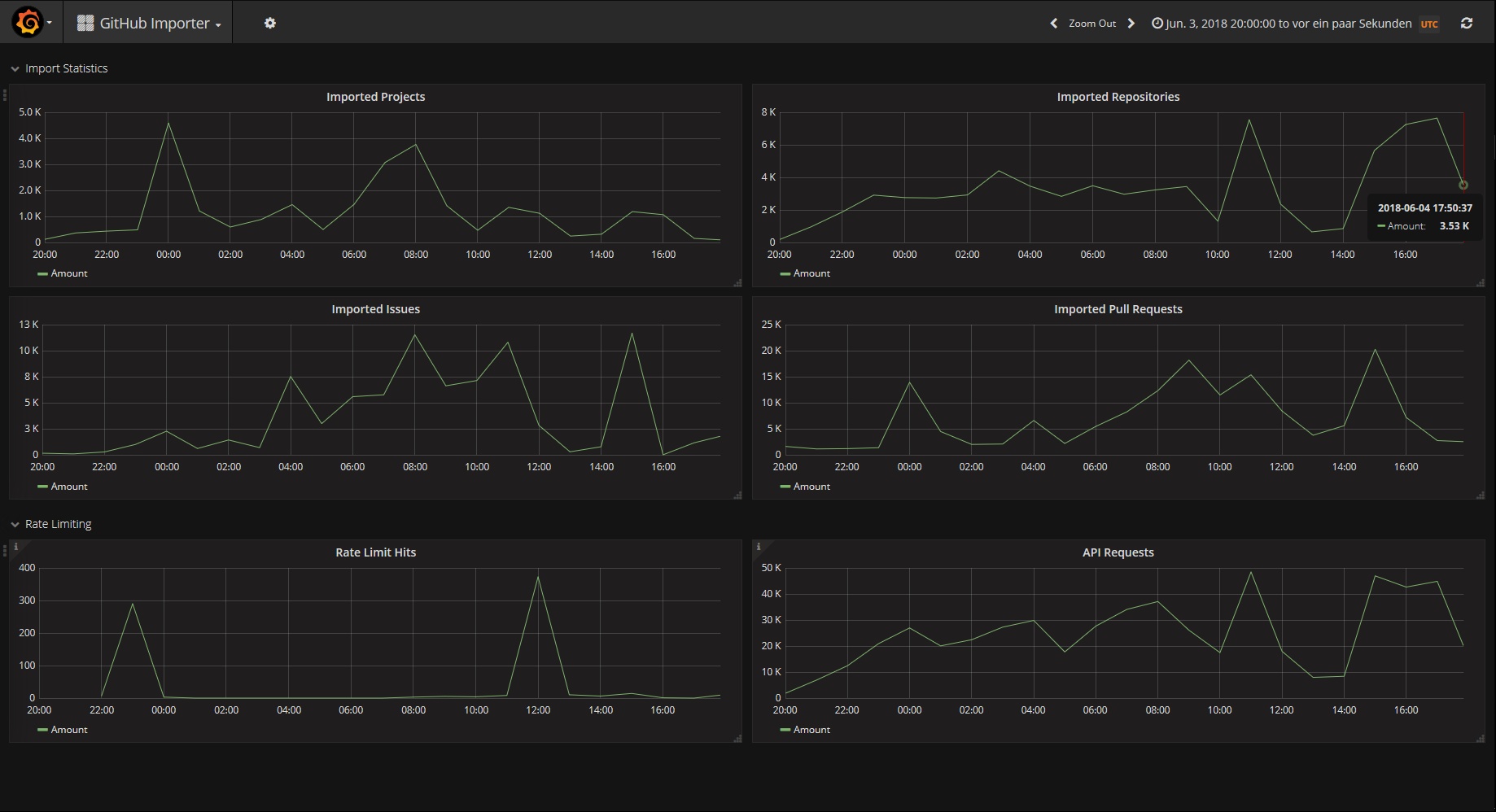
(Screenshot of the GitLab Dashboard for the GitHub Importer on June 4th; Source)
Intrigued by the numbers I immediately wanted to calculate the total of repositories imported from GitHub so far, and I wanted to do this with R. However, it turned out that dealing with JSON is not that easy if you’re working with it for the first time, so it took me a couple of Tweets (and days) to finally come up with an automated approach. This is how I proceeded:
2 Inspect a Website’s DOM & HTTP Requests
My first idea was to extract the data directly from the according HTML object from the dashboard’s source. After navigating through the DOM tree I realized that the data is rendered on a canvas element and therefore is not part of the syntax.
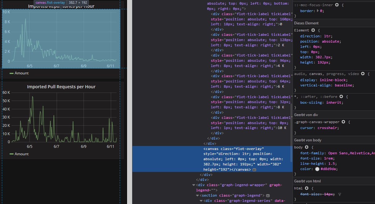
(The dashboard element in the DOM tree. There’s no data in the canvas object.)
We can see that the dashboard is loading the data dynamically (i.e. you can refresh every item) and there are parameters in the URL. This means that there must be some API and GET/POST requests in the site’s HTML.
The formal way would be to consult GitLab’s API documentation…
The quick & dirty way is to locate the request we need directly in the DOM. Just right-click somewhere on the page, open the Web Inspector and switch to the Network Analysis Tab. There you see all the requests being processed when the dashboard is loaded in your browser (you might need to reload the page if the tab is empty).
We’re looking for some queries which return data (most probably XML or JSON), and there you go: The 2nd entry with type: json is the request (and response) for the repositories metric:
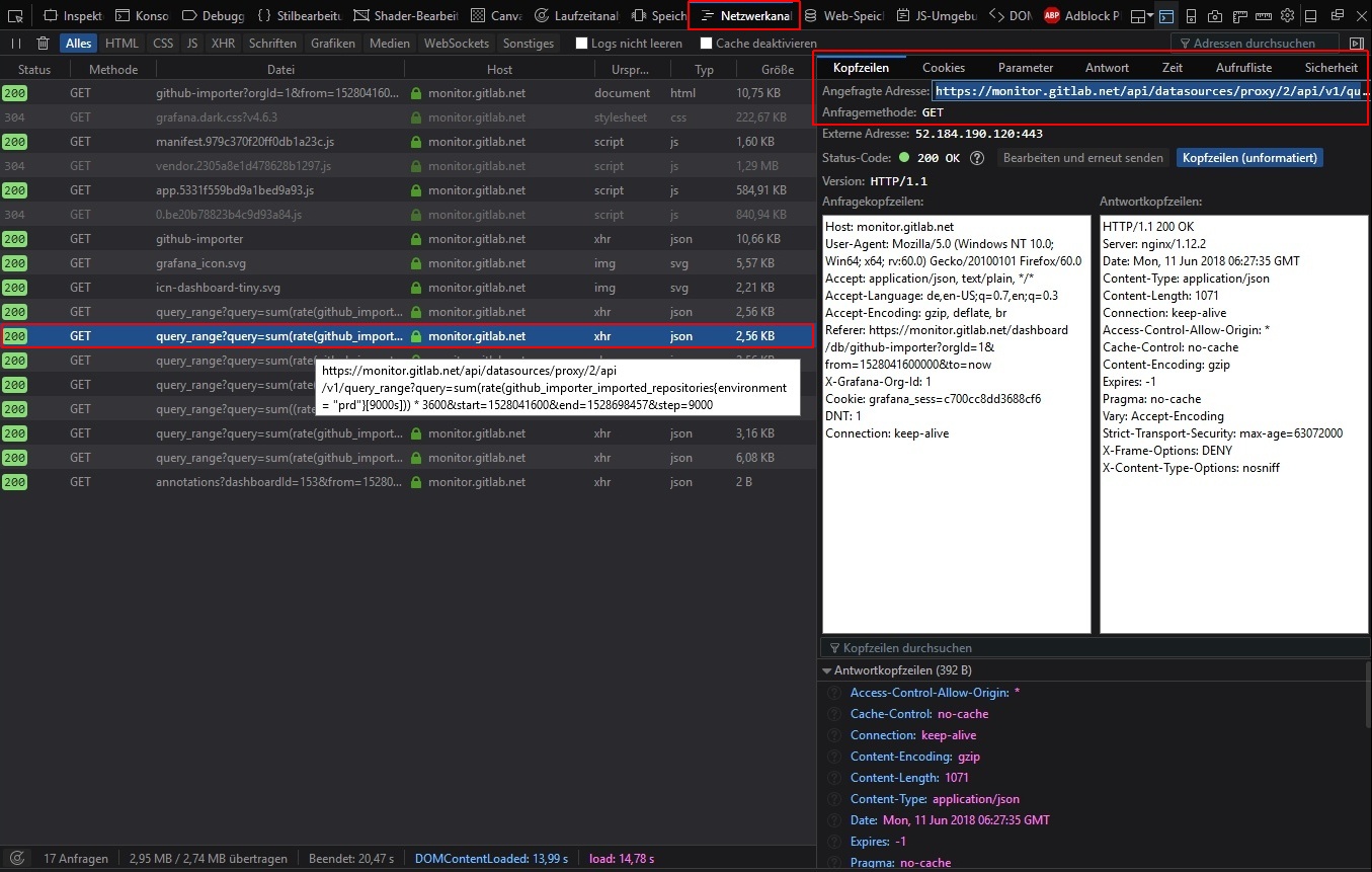
(Screenshot of the Network Analysis Tab in Firefox’ DOM inspector)
3 Extract JSON
3.1 Quick: JSON from File (copy & paste)
If you’re in a hurry, you can copy the JSON data as a string from the response tab, save it as data.json and use the magnificent jsonlite::fromJSON package to get the data into R.
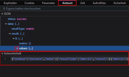
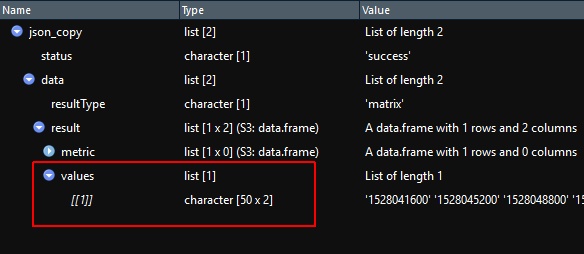
(Direct copy & past access to the JSON data from the query response tab. Fold the values node if you can’t access the content field)
You’ll get a list of nested lists1, have to locate the data node and convert the data into something you can work with (i.e. a tidy data frame). This is the level of insanity where I gave up since I couldn’t manage to iterate over the list without a for-loop:
(*Help!*. I can’t process the atomic level.)
After all, my goal was to find a 2-lines solution in the manners of readr::read_<data_type>, which must not resort to any map_* / transpose() / DataNinja() multi-line (and often: single specific use-case) approaches.
Why is dealing^ with #JSON in #Rstats such a mess? I don’t want a workflow where I have to unnest lists / map_df over nested lists / transpose matrices / subset[ ,1] etc.? There must be an easier way. If not, can we have “read_json” asap please? ^[tried jsonlite and rjson so far]
— Ilja | Илья (@fubits) June 5, 2018
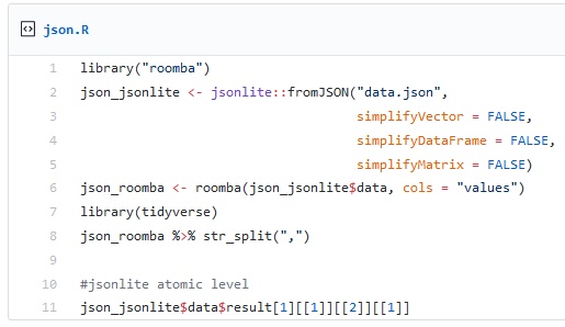
3.1.1 It’s all about [[1]]
Just in case you eventually end up with a similar problem, here’s my (pre-)final 2-lines solution. Addressing the “lastest” list of values with [[1]] eventually did the trick. Since the data in this JSON is stored as n+ pairs of lists nested in a single variable list (values) I either ended up with a single column with all the values or with two rows of strings. The only working solution until then seemed to be @LandonLehman’s suggested double-transpose() approach:
This seems to work. Don't ask me about the multiple transposes - R kept not liking "as_tibble" and this got rid of the errors (maybe using data frame instead would avoid this). Using "rowwise" lets you refer directly to the nested list in that specific row. pic.twitter.com/tzjtj4i4TW
— Landon Lehman (@LandonLehman) June 5, 2018
Also, Maëlle Salmon was so kind to suggest jqr and roomba which both seem very promising but did not get me to the point where I could turn the nested lists into a data frame. You should definitely check out both and follow @ma_salmon.
Only yesterday it somehow struck me that I’m not after the $values variable list, but the list’s unnamed content [[1]]:
(Bummer)
3.1.2 Two Lines, Pt. 1
From here on, it’s rather straightforward:
library(tidyverse) # this line doesn't count.
json_file <- "https://gist.githubusercontent.com/ellocke/498d492dfefd339b8c9884fd07c8f4bb/raw/0efef128bb7dbfe9f3f43c9ce034c6bcdd2ec00a/data.json" # Link to the json.data file in a Gist

# Two lines
json_copy <- jsonlite::fromJSON(json_file)
json_copy$data$result$values[[1]] %>% as.tibble() %>% head(5)
Notice that the values are processed as character strings… We’ll deal with this in a second. Same for the V1 variable which actually is date & time in the Unix Timestamp format aka
POSIX.
Ok, that’ll basically suffice for a quick analysis, but if you want to automate fetching the JSON data from an API instead of manually copying & pasting it every time you update your analysis, there’s only one way: We need to automate the GET request from within R.
3.2 Robust: Fetch JSON from API with GET
First, we need the httr-package, which is a convenient wrapper for lots of common HTTP / curl methods. Check out the vignette for httr.
library(httr)Next, we need the query as an URL which we can grab from the Network Analysis tab (see above).
DOM_URL <- parse_url('https://monitor.gitlab.net/api/datasources/proxy/2/api/v1/query_range?query=sum(rate(github_importer_imported_repositories{environment = "prd"}[9000s])) * 3600&start=1528041600&end=1528698457&step=9000') # we either need to escape "prd" with \"prd\" or use ' ' for the outer string wrapping

json_raw <- GET(url = DOM_URL)
http_status(json_raw)$message # let's check if the GET request was a success (=200)
# content(json_dom, "parsed") # one way to see the content
3.3 Parse JSON
Now we need to parse the content we received from the request to something we can further process. Right now, the $content node is literally raw:
# json_raw$content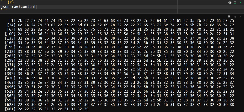
(Rawrrrrrr)
Let’s parse it. httr offers a couple of convenient shortcuts here. We can parse the JSON as a String (with as = "text") and then process it with jsonlite::fromJSON. Or we can instantly parse it to “parsed”" JSON with 1 line. (Not working properly for me, yet)
# as = "text"
json_parsed <- content(json_raw, as = "text") # simple, for follow-up with jsonlite::fromJSON()
# str(json_parsed)

#  as = "parsed"
# json_object <- content(json_raw, as = "parsed", type = "application/json", encoding = "UTF-8")
## this forces us to use something like
## json_object$data$result[[1]]$values %>%
##    transpose() %>%
##      {do.call(cbind,.)} %>%
##      as.tibble() %>%
##      unnest()
## OR
## json_object$data$result[[1]]$values %>%
##      transpose() %>%
##      set_names(c("date", "value")) %>%
##      as.tibble() %>%
##      unnest()
## HORRIBLE!
4 From JSON to Tidy
Now - either on the JSON string or the JSON object (list of lists) - we just need to %>% as.tibble()
json_object <- jsonlite::fromJSON(json_parsed) # (if parsed with 'as = "text"')
json_object$data$result$values[[1]] %>% as.tibble() -> json_dirty
# json_object$data$result[[1]][[2]] %>% as.tibble() -> json_dirty # not working, yet
# json_object[["data"]][["result"]][[1]][["values"]] %>% as.tibble() # not working, yet
head(json_dirty, 5) #> 2x chr
As both columns/variables are coded as character strings - and we want to have the first column as a Date type variable - we’d need to use mutate on both. Furthermore, lubridate::as_datetime is of insane value here but needs something numeric, too. We actually have Unix Timestamp data here which would be something * something * 86400 seconds if you wanted to convert it to a human readable format. as_datetime() simply does it with one call.
4.1 Tidy Date #1 with lubridate
json_dirty %>%
  mutate(V1 = lubridate::as_datetime(as.numeric(V1)), # first to int, then to date
         V2 = as.numeric(V2)) -> json_tidy
head(json_tidy)
However, we can simplify this even further!
4.2 Tidy Date #2: type_convert() to the Rescue / Two Lines, Pt. 2
# json_object <- jsonlite::fromJSON(json_parsed)
json_object$data$result$values[[1]] %>% as.tibble() %>% type_convert() -> json_dirty
head(json_dirty, 5) # > int & dbl
Now the date & time / POSIX column:
json_dirty %>%
  mutate(V1 = lubridate::as_datetime((V1))) -> json_tidy
head(json_tidy) # > V1 == <dttm>
Ok, almost done. Let’s rename the variables to something meaningful with rename() and finally plot the data
(Yes, we could also have used
json_tidy %>% mutate(date = V1, repos = V2) %>% select(-V1, -V2)
but rename() seems more efficient here.
json_tidy %>% rename(date = V1, repos = V2) -> json_tidy5 Plots
5.1 Hourly # of Repos migrated from GitHub to GitLab
json_tidy %>%
  ggplot(aes(x = date, y = repos)) +
  geom_line()
5.2 Total # of Repos, cumulated over Time
json_tidy %>%
  ggplot(aes(x = date, y = repos)) +
    geom_line(aes(y = cumsum(repos)))
5.3 Bonus: GitHub API Rate Limit Hits
Same procedure as above:
- find the request’s URL
- fetch with
httr, parse withjsonlite - tidy with
dplyr& plot withggplot
GET the Query
DOM_URL_rates <- parse_url('https://monitor.gitlab.net/api/datasources/proxy/2/api/v1/query_range?query=sum(rate(github_importer_rate_limit_hits%7Benvironment%3D%22prd%22%7D%5B3600s%5D))%20*%203600&start=1528041600&end=1528698457&step=3600') # we either need to escape "prd" with \"prd\" or use ' ' for the outer string wrapping
json_rates <- GET(url = DOM_URL_rates)
# http_status(json_rates)
# content(json_dom, "parsed")
Parse JSON
Now that we know how deal with the JSON output we can actually do the processing in a single working step.
Technically, without intending this would fit in two lines of code :)
json_rates <- content(json_rates, "text", encoding = "UTF-8") # UTF-8 == default
jsonlite::fromJSON(json_rates)$data$result$values[[1]] %>%
  as.tibble() %>%
  type_convert() %>%
  mutate(V1 = lubridate::as_datetime(V1)) %>%
  rename(date = V1, limit_hits = V2) -> json_rates
5.4 Plot # of Repos & GitHub API Rate Limit Hits
ggplot() +
  geom_line(data = json_tidy, aes(x = date, y = repos), color = "blue") +
  geom_line(data = json_rates, aes(x = date, y = limit_hits), color = "red")
Done! Actually, not that hard right? Only took me a couple of days to figure this out… I’ll update this post as soon as I have found a more efficient way (in lines of code).
6 Update: Further Reading
Oscar Lane just published a more generalized approach to mining data from “Browser-based” APIs: “Reverse engineering web APIs for scraping”
His
map_*-approach to JSON looks very efficient:
An analogy I came up with while writing this is think of arriving at the last node - but actually you need the “lastest”. This is a reference to the German miss-term Einzigste which is a superlative of the superlative for “the one and only” which would be something like “the one and onlyest”.↩