[R] German Academic Twitter, Pt. 1: Mining #dvpw18, #dgs18, #hist18, #informatik2018 et al.
Abstract / TL;DR
Updated: In September, five big academic societies in Germany had their annual meetings - all at the same time! You can **not not** harvest their tweets. I'll explain step-by-step how to mine them with rtweet and how to wrangle the Tweets for a tidy analysis.
- 1 Setting: The Big 5 on Twitter
- 2 Preparation
- 3 Mining Tweets with
search_tweets() - 4 Some Comparisons
- 5 Final scores: The overall activity compared by numbers
- 6 What’s next?
1 Setting: The Big 5 on Twitter

Update 3: As I’ve stumbled upon some irregularities in my follow-up post, it turned out that the Twitter sample for the Sociology conference (esp.
#dgs2018) was heavily cross-poluted by another popular event using the same Hashtag in Turkey… This has been adressed in the follow-up post,but has yet to be implemented hereand now is also adjusted for in this post.
Update 2: The Media Studies conference (#gfm2018) has been included
Update: Since the conferences are over but there’s still some Twitter activity, Tweets posted after 29.09.2018 have been filtered out from the samples.
As (bad) luck has it, four five big academic societies in Germany somehow decided to hold their respective annual meetings within the same week:
Deutsche Vereinigung für Politikwissenschaft / Political Science (#dvpw18, #dvpw2018, #dvpw)
Deutsche Gesellschaft für Soziologie / Sociology (#dgs18, #dgs2018)
Verband der Historiker und Historikerinnen Deutschlands / History (#histag18 / #histag2018 / #historikertag2018)
- Gesellschaft für Informatik e.V. / Computer Science (#informatik2018)
Gesellschaft für Medienwissenschaft / Media Studies (#gfm2018)
Even though Germany is still a bit behind with regards to Twitter, four five conferences = 4x 5x the chance to work on your Twitter mining and text wrangling skills ;). Plus, we get some interesting data for the future practice of our NLP / text processing and social network analysis skills…
So let’s just get started with mining. We will use Mike Kearney’s superb rtweet (package).
library(tidyverse)
library(here)
library(rtweet)
2 Preparation
2.1 Setting up rtweet
Get the Token
Follow the instructions here, set up your Twitter app and save your token.
You’ll get something like this (caution: fake credentials)
appname <- "your_app_name"
key <- "your_consumer_key"
secret <- "your_seceret"
Register your App with R.
twitter_token <- create_token(
  app = appname,
  consumer_key = key,
  consumer_secret = secret)
And save your token in your environment / home path / working directory.
Save token in Root dir / Home path
## path of home directory
home_directory <- path.expand("~/R")
file_name <- file.path(home_directory, "twitter_token.rds")

## save token to home directory
saveRDS(twitter_token, file = file_name)
# saveRDS(twitter_token, "twitter_token.rds") # save locally in wd
twitter_token <- readRDS(str_c(home_directory,"/twitter_token.rds"))
Token check
identical(twitter_token, get_token())
#> TRUE
2.2 getTimeString() Helper Function
I will use this function for saving time-stamped samples of Tweets
getTimeString <- function() {
  Sys.time() %>% str_extract_all(regex("[0-9]")) %>%
    unlist() %>% glue::glue_collapse()
  }
getTimeString()
## 201811181512422.3 (Prepare filepath for .rds with here())
# library(here) # https://blogdown-demo.rbind.io/2018/02/27/r-file-paths/
# blogdown-specific work-around for the `data`-folder
data_path <- here("data", "ConferenceTweets", "/")
if (!dir.exists(data_path)) dir.create(data_path)
# saveRDS(mtcars, str_c(data_path, "test", ".rds")) # test filepath
# readRDS(str_c(data_path, "test", ".rds")) # test filepath
3 Mining Tweets with search_tweets()
We probably won’t get all the tweets with a single request, so what we are going to do is, to request the Tweets multiple times, consolidate the requests, and finally extract unique Tweets with dplyr::distinct() to get a pretty good sample.
Notice, that we can request recent and mixed samples (However, popular doesn’t seem to work for me, atm.)
3.1 Political Science: #dvpw18 / #dvpw2018 (and #dvpw)
3.1.1 Mining
The workflow suggested here is that you mine a couple of samples (or mine new samples hours or days later), save these samples with time-stamped and therefore unique file names (as group_timestamp.rds), and than consolidate and extract unique tweets with dplyr::distinct()
dvpw_tweets <- search_tweets(q = "#dvpw18 OR #dvpw2018 OR #dvpw", # explicit QUERY
      include_rts = FALSE,
      # max_id = ,
      n = 5000,
      verbose = TRUE,
      retryonratelimit = TRUE,
      type = "recent") # mixed recent (popular)

saveRDS(dvpw_tweets, file =
          str_c(data_path,"dvpw_tweets_", getTimeString(),".rds"))
3.1.2 Wrangling
Here we’ll get a file list of all dvpw_*.rds files, then map_dfr() them to a data_frame and finally extract unique Tweets with distinct()
## this is just a bit complicated because I'm using an external data folder for blogdown. If you work locally, you can just use:
# map_dfr(dir(path = ".", "dvpw_"), readRDS)

dvpw_rds <- dir(path = data_path, pattern = "dvpw_") %>%
  str_c(data_path, .) %>%
  map_dfr(readRDS)
dvpw_collection <- dvpw_rds %>%
  distinct(status_id, .keep_all = TRUE) %>%
  filter(created_at > "2018-09-23" &
         created_at < "2018-09-30") %>%
  arrange(created_at)
As you can see from
filter(created_at < "2018-09-30")we will only consider tweets posted before Sunday, 30.09.2018 (for the sake of comparison)
(How to check the latest/earliest Tweet)
min(dvpw_collection$status_id) # https://twitter.com/statuses/1041748634486931465
Tweet <- max(dvpw_collection$status_id)
browseURL(str_c("https://twitter.com/statuses/", Tweet))
Time-String for Plotting
timeString <- str_c(lubridate::hour(Sys.time()), ":", lubridate::minute(Sys.time()))3.1.3 Treemap: #dvpw / #dvpw18 / #dvpw2018
We’ll need the treemapify package for this.
dvpw_n_tweets <- nrow(dvpw_collection)
dvpw_n_accounts <- length(unique(dvpw_collection$screen_name))
# tidy/dplyr: distinct(screen_name) %>% count()

dvpw_collection %>%
  group_by(screen_name) %>%
  summarise(n = n()) %>%
  mutate(share = n / sum(n)) %>%
  arrange(desc(n)) %>%
  ggplot(aes(area = share)) +
    treemapify::geom_treemap(aes(fill = log10(n))) +
    treemapify::geom_treemap_text(
      aes(label = paste0(screen_name, " (", round(share*100,1),"%)"))
      ) +
  scale_fill_viridis_c(direction = -1, option = "C", begin = 0.8) +
  labs(title = "Twitter-Aktivität zu #dvpw / #dvpw18 / #dvpw2018",
       subtitle = paste0("(n = ", dvpw_n_tweets,
                         " Tweets von m = ", dvpw_n_accounts,
                         " Accounts; Stand: 29.09.18, ",
                         "23:59" , " Uhr;",
                         " by @fubits)")) +
  guides(fill = FALSE)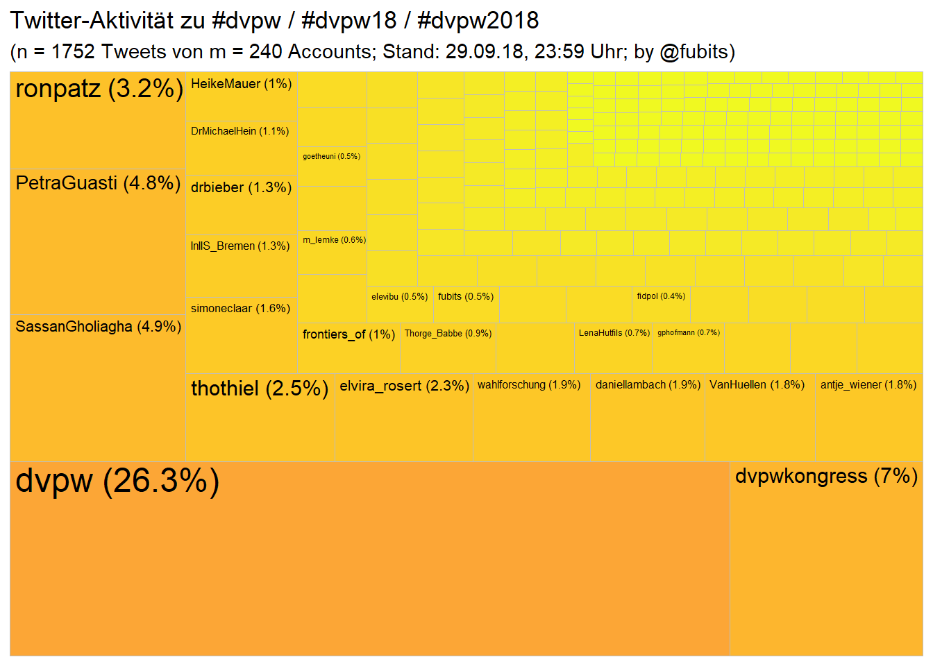
3.1.4 Scatterplot: # of Tweets / RTs / Favs per User
For the scatterplot we’ll have to group the single Tweets by user ($screen_name), summarise the counts for Tweets, RTs, and Favs, and assign a “discipline” category for later use.
dvpw_counts <- dvpw_collection %>%
  group_by(screen_name) %>%
  summarise(Tweets = n(),
            RT = sum(retweet_count),
            Favs = sum(favorite_count)) %>%
  mutate(discipline = "PolSci") %>%
  arrange(desc(Tweets)) # %>%
  # top_n(n = 50, wt = tweets)
Scatterplot
ggplot(dvpw_counts, aes(x = Favs, y = RT)) +
  geom_point(aes(size = Tweets, color = screen_name)) +
  ggrepel::geom_text_repel(data = dvpw_counts[1:2,], aes(label = screen_name)) +
  coord_fixed() +
  scale_color_viridis_d() +
  scale_x_continuous(breaks = scales::pretty_breaks(6)) +
  guides(color = FALSE) +
  theme_minimal() +
  labs(size = "Anzahl Tweets",
       title = "Twitter-Aktivität zu #dvpw / #dvpw18 / #dvpw2018: Retweets & Favs",
       subtitle = paste0("(n = ", dvpw_n_tweets,
                       " Tweets von m = ", dvpw_n_accounts,
                       " Accounts; Stand: 29.09.18, ", "23:59" , " Uhr;"),
       x = "Anzahl Favourites",
       y = "Anzahl Retweets",
       caption = "@fubits")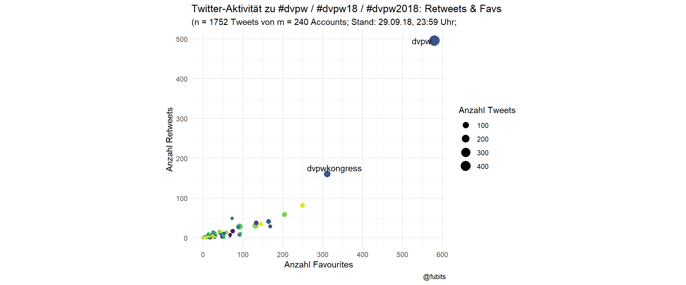
The official society accounts have been quite busy! Well done, @dvpw/@dvpwkongress, the idea of a Twitter #TeamTakeOver worked out rather well! <- Note to my future self.)
To be precise, the collective action of
@dvpwhas produced n = 460 individual Tweets!
3.1.5 Scatterplot without @dvpw and with labels for the top 20
Here we’ll need ggrepel for non-overlapping labelling. As the official @dvpw account has been quite an “outlier”, let’s have an undisturbed look at the rest of the field without @dvpw.
dvpw_counts %>% filter(screen_name != "dvpw") %>%
  ggplot(aes(x = Favs, y = RT)) +
    geom_point(aes(size = Tweets, color = screen_name), alpha = 0.5) +
    ggrepel::geom_text_repel(data = dvpw_counts[2:21,],
                             aes(label = screen_name)) +
    coord_fixed() +
    scale_color_viridis_d() +
    scale_x_continuous(breaks = scales::pretty_breaks(6)) +
    guides(color = FALSE) +
    theme_minimal() +
    labs(size = "Anzahl Tweets",
         title = "Twitter-Aktivität zu #dvpw / #dvpw18 / #dvpw2018: Top 20 Accounts (ohne @dvpw)",
         subtitle = paste0("(n = ",
                           sum(filter(dvpw_counts,
                                      screen_name != "dvpw")$Tweets),
                           " Tweets von m = ", dvpw_n_accounts - 1,
                         " Accounts, ohne @dvpw; Top 20 Label, Stand: 29.09.18, ",
                         "23:59"," Uhr)"),
         x = "Anzahl Favourites",
         y = "Anzahl Retweets",
         caption = "@fubits")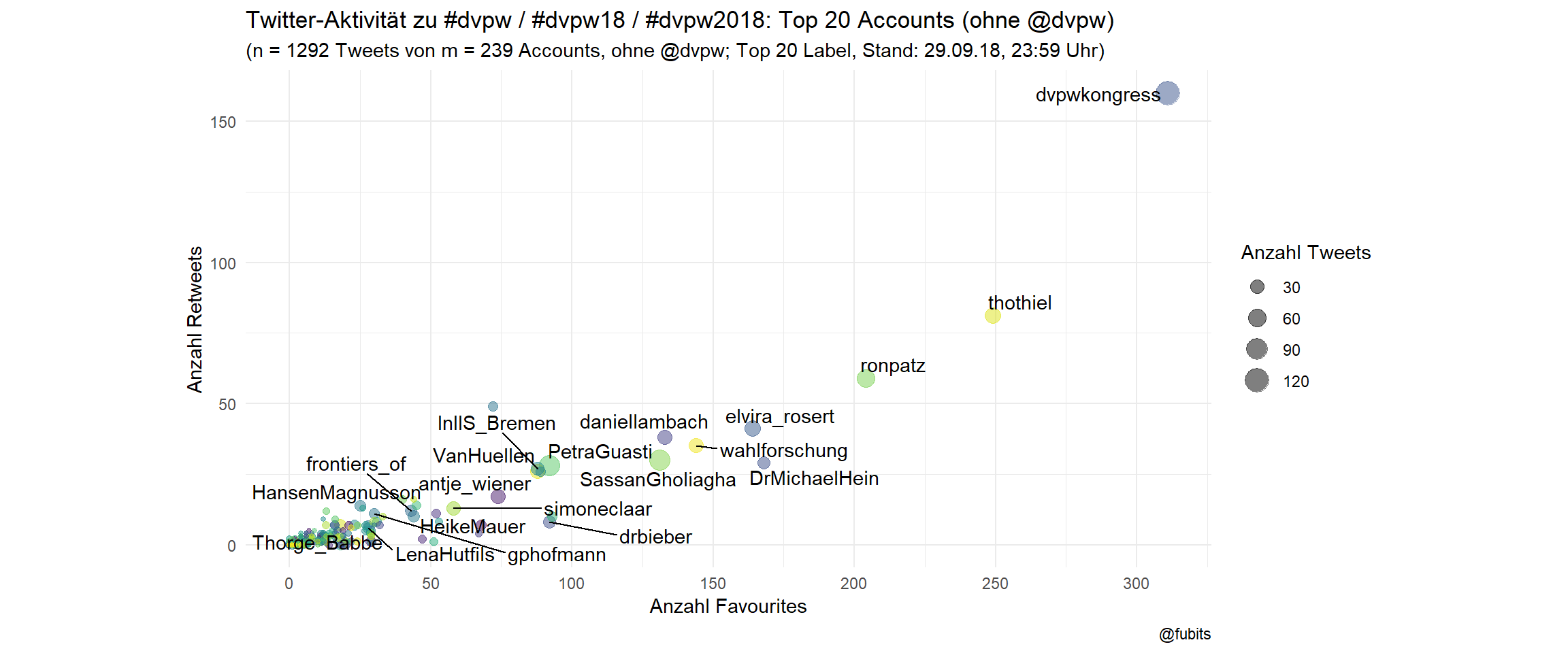
3.1.6 (TODO: Creating Twitter Lists)
tba, but we could automate creating of user lists from hashtags for conferences… This might be useful for live-curating Twitter handles for better credits to speakers.
# we need a plain character vector here
dvpw_nicks <- dvpw_collection %>% distinct(screen_name) %>% unlist()
post_list(dvpw_nicks[1:100], name = "dvpw2018", private = TRUE, destroy = FALSE)
#> Can only add 100 users at a time. Adding users[1:100]...
list_length <- length(dvpw_nicks)
post_list(dvpw_nicks[101:200], slug = "dvpw2018", private = TRUE, destroy = FALSE)
post_list(dvpw_nicks[200:length(dvpw_nicks)], slug = "dvpw2018", private = TRUE, destroy = FALSE)

# delete with
# post_list(slug = "dvpw2018", destroy = TRUE)
3.2 Sociology: #dgs18 / #dgs2018 (UPDATE!)
Let’s have a look at how German Sociologists performed on Twitter. Like above, I’ve mined the Tweets multiple times in order to get a good sample.
Mine
dgs_tweets <- search_tweets(q = "#dgs18 OR #dgs2018", # explicit QUERY
      include_rts = FALSE,
      # max_id = ,
      n = 5000,
      verbose = TRUE,
      retryonratelimit = TRUE,
      type = "recent") # mixed recent (popular)

saveRDS(dgs_tweets,
        file =  str_c(data_path,"dgs_tweets_", getTimeString(),".rds"))
Wrangle
dgs_rds <- dir(path = data_path, pattern = "dgs_") %>%
  str_c(data_path, .) %>%
  map_dfr(readRDS)
As I have discovered some irregularities while pre-processing the Tweets for a corpus analysis (see the follow-up post for details), the Sociology Twitter sample needs extra-filtering. Consequently, all the following analyses and plots have been re-done and updated.
As we can see from the following time-series plot, the #dgs2018 hashtag has, first been used by the Turkish community before German Sociologists took over around the 23th:
dgs_rds %>% distinct(status_id, .keep_all = TRUE) %>%
  filter(created_at < "2018-09-30") %>%
  filter(lang == "tr" | lang == "de") %>%
  group_by(lang) %>%
  rtweet::ts_plot() +
    theme_minimal()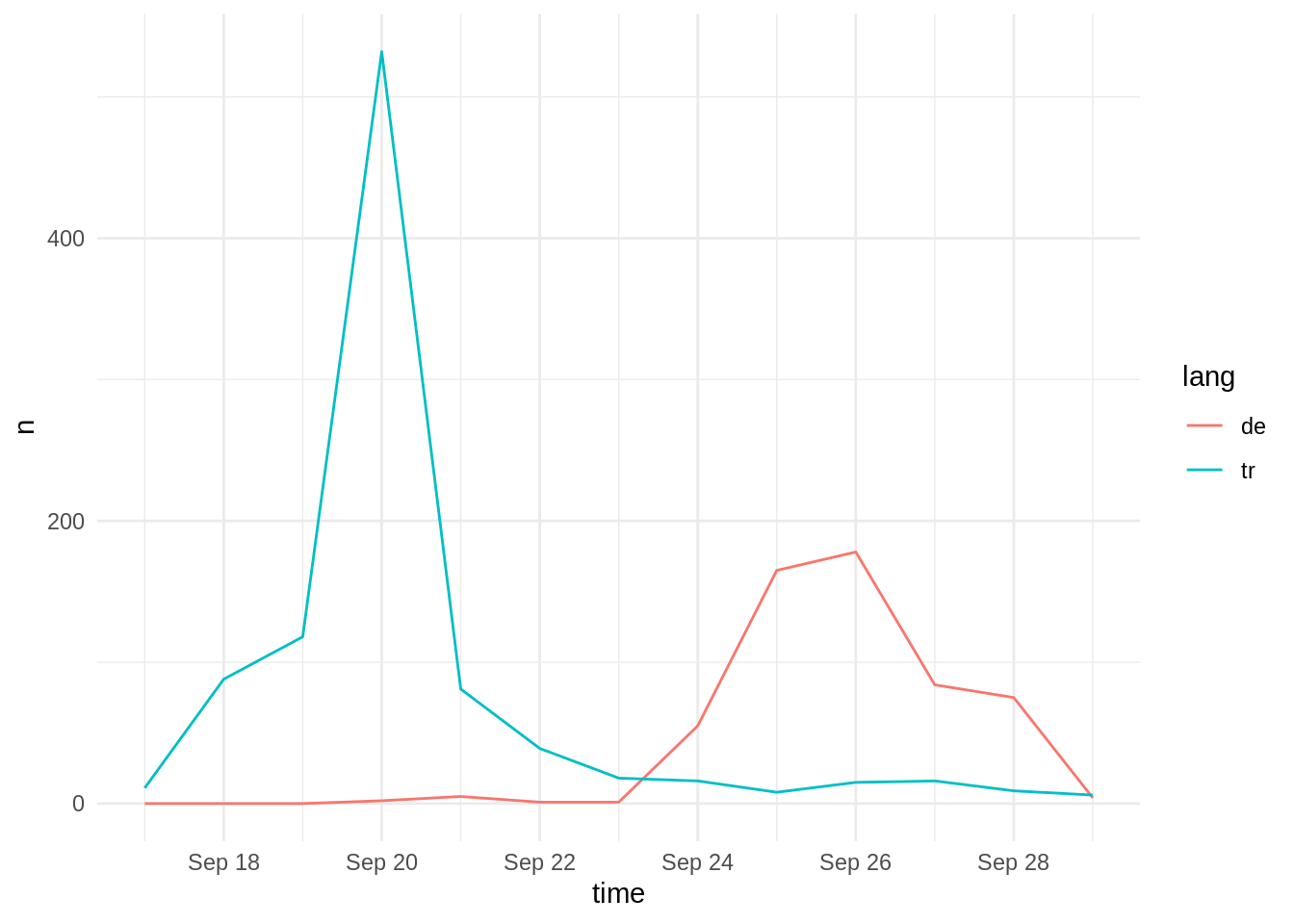
Therefore, we have to do two things: narrow down the time period to 23.9.-29.9. and filter out as many Turkish accounts as possible.
For the sake of comparability, 23.9. has been set as the lower limit for the other disciplines, too.
# ID TR users
tr_user <- dgs_rds %>%
  distinct(status_id, .keep_all = TRUE) %>%
  filter(lang == "tr") %>%
  select(user_id) %>%
  distinct()

## Syntax for hand-picking suspicious hashtags
# dgs_collection %>%
#   filter(lang == "und") %>%
#   filter(!str_detect(text,"yks2018|yksdil|dgsankara|cumhuriyetüniversitesi|DanceKafe")) %>%
#   select(screen_name,text)

# ID lang=="und" Tweets with certain hashtags ("yks2019", "yksdil", ...)
und_user <- dgs_rds %>%
  distinct(status_id, .keep_all = TRUE) %>%
  filter(str_detect(text,"yks2018|yksdil|dgsankara|
                     cumhuriyetüniversitesi|DanceKafe")) %>%
  select(user_id) %>%
  distinct()

# limit time period
dgs_collection <- dgs_rds %>%
  distinct(status_id, .keep_all = TRUE) %>%
  filter(lang != "tr") %>%
  filter(created_at > "2018-09-23" &
         created_at < "2018-09-30") %>%
  arrange(created_at)

#remove TR users from collection
dgs_collection <- dgs_collection %>%
  anti_join(bind_rows(tr_user,und_user), by = "user_id")
Sociology: Treemap
dgs_n_tweets <- nrow(dgs_collection)
dgs_n_accounts <- length(unique(dgs_collection$screen_name))
dgs_collection %>%
group_by(screen_name) %>%
summarise(n = n()) %>%
mutate(share = n / sum(n)) %>%
arrange(desc(n)) %>%
ggplot(aes(area = share)) +
treemapify::geom_treemap(aes(fill = log10(n))) +
treemapify::geom_treemap_text(
aes(label = paste0(screen_name, " (", round(share*100,1),"%)"))
) +
scale_fill_viridis_c(direction = -1, option = "C", begin = 0.8) +
labs(title = "Twitter-Aktivität zu #dgs18 / #dgs2018 (UPDATE)",
subtitle = str_c("(n = ", dgs_n_tweets,
" Tweets von m = ", dgs_n_accounts,
" Accounts; Stand: 29.09.18, ", "23:59" , " Uhr;",
" by @fubits)")) +
guides(fill = FALSE)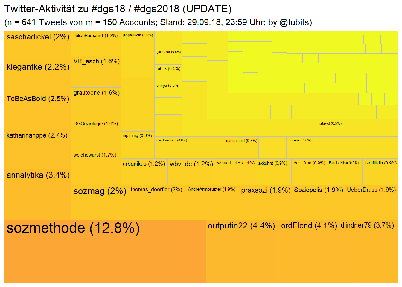 That looks rather different from the #dvpw2018 community. Less institutional dominance and
 actually, many more less individual Twitter users (150 active users vs 240 in team PolSci).
just for comparison, here’s what my first bad take looked like: 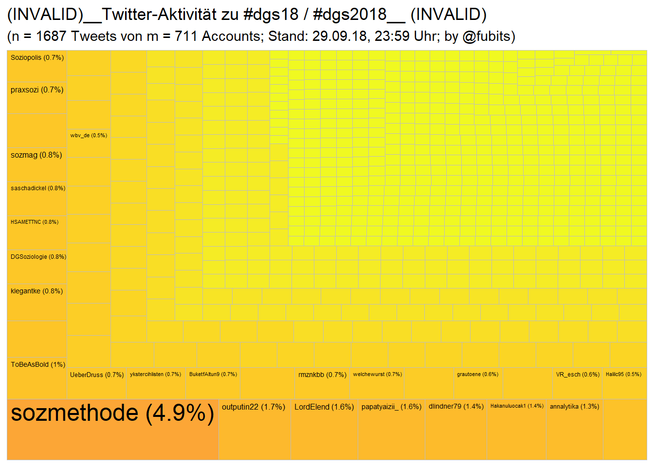
So, unfortunately, after removing all the Turkish
#dgs2018we’re down from initially 1687 to 641 unique Tweets from 150 unique Users (instead of 711)…
Sociology: per-User
dgs_counts <- dgs_collection %>%
  group_by(screen_name) %>%
  # filter(screen_name != "fubits") %>%
  summarise(Tweets = n(),
            RT = sum(retweet_count),
            Favs = sum(favorite_count)) %>%
  mutate(discipline = "Sociology") %>%
  arrange(desc(Tweets)) # %>%
  # top_n(n = 50, wt = tweets)
ggplot(dgs_counts, aes(x = Favs, y = RT)) +
geom_point(aes(size = Tweets, color = screen_name)) +
# ggrepel::geom_text_repel(data = counts[1:10,], aes(label = screen_name)) +
coord_fixed() +
scale_color_viridis_d() +
scale_x_continuous(breaks = c(10,20,30,40,50,75,100,150,175)) +
guides(color = FALSE) +
theme_minimal() +
labs(size = "Anzahl Tweets",
title = "Twitter-Aktivität zu #dgs18 / #dgs2018: Retweets & Favs (UPDATE)",
subtitle = paste0("(n = ", dgs_n_tweets,
" Tweets von m = ", dgs_n_accounts,
" Accounts; Stand: 29.09.18, ", "23:59" , " Uhr;"),
x = "Anzahl Favourites",
y = "Anzahl Retweets",
caption = "@fubits")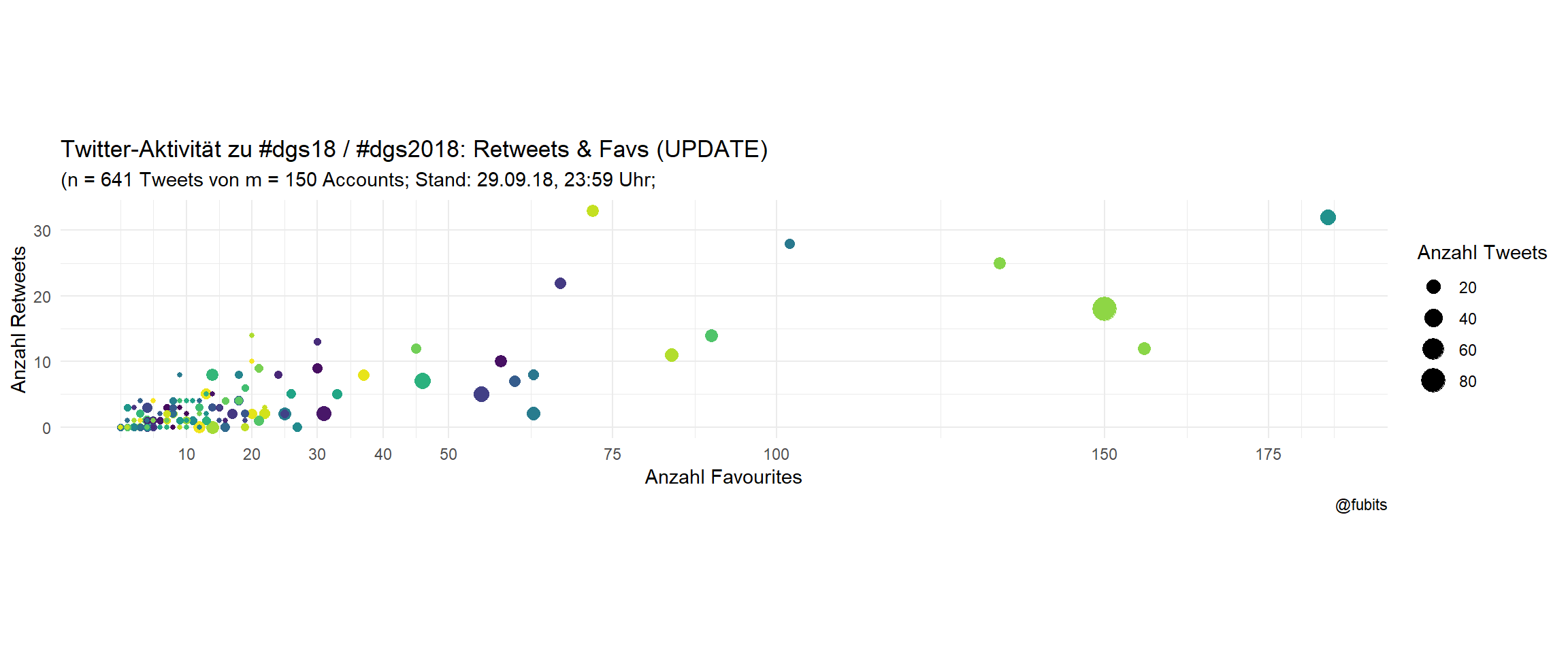
So, that is quite different from PolSci, right? Less individual tweets per user, less retweets, but a significantly higher Fav rate. Interesting. Shall we assume that Sociologist are more introvert and maybe have more empathy for others? :)
Sociology: Top 20 labelled
ggplot(dgs_counts, aes(x = Favs, y = RT)) +
    geom_point(aes(size = Tweets, color = screen_name), alpha = 0.5) +
    ggrepel::geom_text_repel(data = dgs_counts[1:20,],
                             aes(label = screen_name)) +
    coord_fixed() +
    scale_color_viridis_d() +
    scale_x_continuous(breaks = c(10,20,30,40,50,75,100,150,175)) +
    guides(color = FALSE) +
    theme_minimal() +
    labs(size = "Anzahl Tweets",
         title = "Twitter-Aktivität zu #dgs18 / #dgs2018: Top 20 Accounts (UPDATE)",
         subtitle = paste0("(n = ", dgs_n_tweets,
                         " Tweets von m = ", dgs_n_accounts,
                         " Accounts; Top 20 Label, Stand: 29.09.18, ",
                         "23:59", " Uhr)"),
         x = "Anzahl Favourites",
         y = "Anzahl Retweets",
         caption = "@fubits")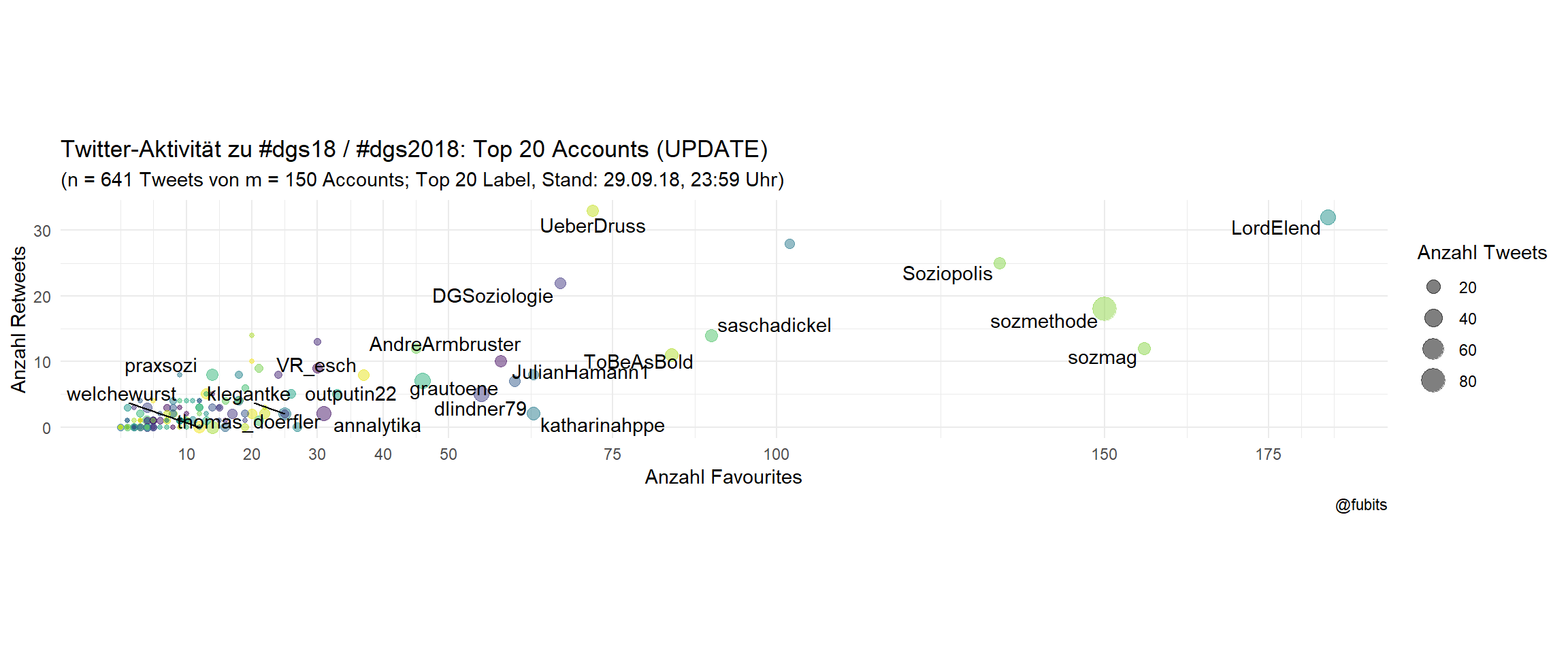
3.3 Historians: #histag18 / #histag2018 / #historikertag2018
Next, let’s look have at the Twitter activity of German History scholars.
Mine
hist_tweets <- search_tweets(q = "#histag18 OR #histag2018 OR #historikertag2018", # explicit QUERY
      include_rts = FALSE,
      # max_id = ,
      n = 5000,
      verbose = TRUE,
      retryonratelimit = TRUE,
      type = "mixed") # mixed recent popular

saveRDS(hist_tweets, file =
          str_c(data_path,"hist_tweets_",getTimeString(),".rds"))
Wrangle
hist_rds <- dir(path = data_path, pattern = "hist_") %>%
  str_c(data_path, .) %>%
  map_dfr(readRDS)
hist_collection <- hist_rds %>%
  distinct(status_id, .keep_all = TRUE) %>%
  filter(created_at > "2018-09-23" &
         created_at < "2018-09-30") %>%
  arrange(created_at)
Historians: Treemap
hist_n_tweets <- nrow(hist_collection)
hist_n_accounts <- length(unique(hist_collection$screen_name))

hist_collection %>%
  group_by(screen_name) %>%
  summarise(n = n()) %>%
  mutate(share = n / sum(n)) %>%
  arrange(desc(n)) %>%
  ggplot(aes(area = share)) +
    treemapify::geom_treemap(aes(fill = log10(n))) +
    treemapify::geom_treemap_text(
      aes(label = paste0(screen_name, " (", round(share*100,1),"%)"))
      ) +
  scale_fill_viridis_c(direction = -1, option = "C", begin = 0.8) +
  labs(title = "Twitter-Aktivität zu #histag18 / #histag2018 / #historikertag2018",
       subtitle = paste0("(n = ", hist_n_tweets,
                         " Tweets von m = ", hist_n_accounts,
                         " Accounts; Stand: 29.09.18, ", "23:59" , " Uhr;",
                         " by @fubits)")) +
  guides(fill = FALSE)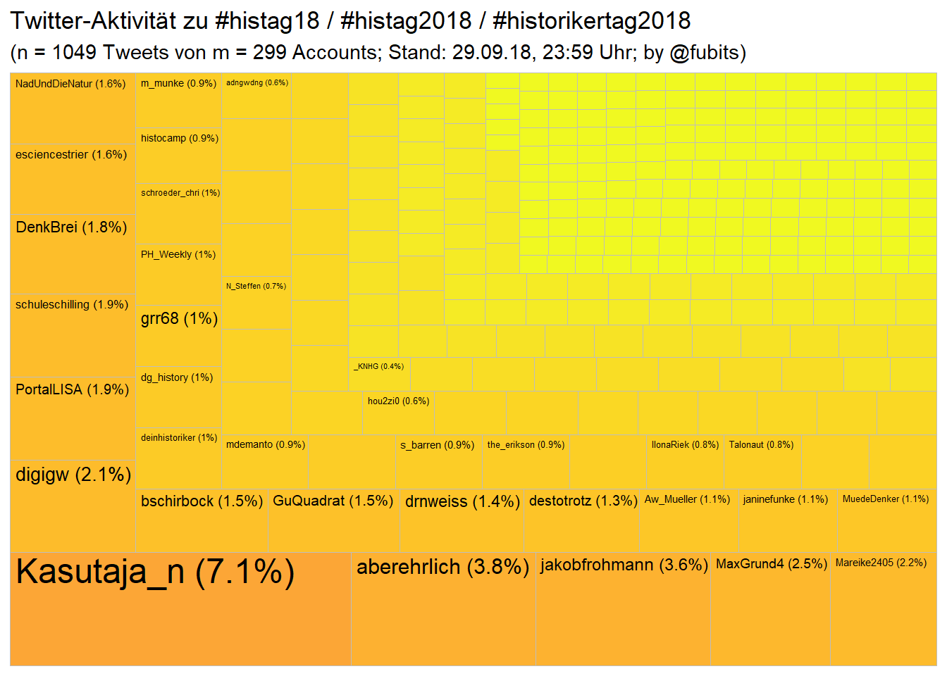
Historians: per-User
hist_counts <- hist_collection %>%
  group_by(screen_name) %>%
  # filter(screen_name != "fubits") %>%
  summarise(Tweets = n(),
            RT = sum(retweet_count),
            Favs = sum(favorite_count)) %>%
  mutate(discipline = "History") %>%
  arrange(desc(Tweets)) # %>%
  # top_n(n = 50, wt = tweets)
ggplot(hist_counts, aes(x = Favs, y = RT)) +
geom_point(aes(size = Tweets, color = screen_name)) +
# ggrepel::geom_text_repel(data = counts[1:10,], aes(label = screen_name)) +
coord_fixed() +
scale_color_viridis_d() +
scale_x_continuous(breaks = scales::pretty_breaks(6)) +
guides(color = FALSE) +
theme_minimal() +
labs(size = "Anzahl Tweets",
title = "Twitter-Aktivität zu #histag18 / #histag2018 / #historikertag2018: Retweets & Favs",
subtitle = paste0("(n = ", hist_n_tweets,
" Tweets von m = ", hist_n_accounts,
" Accounts; Stand: 29.09.18, ", "23:59" , " Uhr;"),
x = "Anzahl Favourites",
y = "Anzahl Retweets",
caption = "@fubits")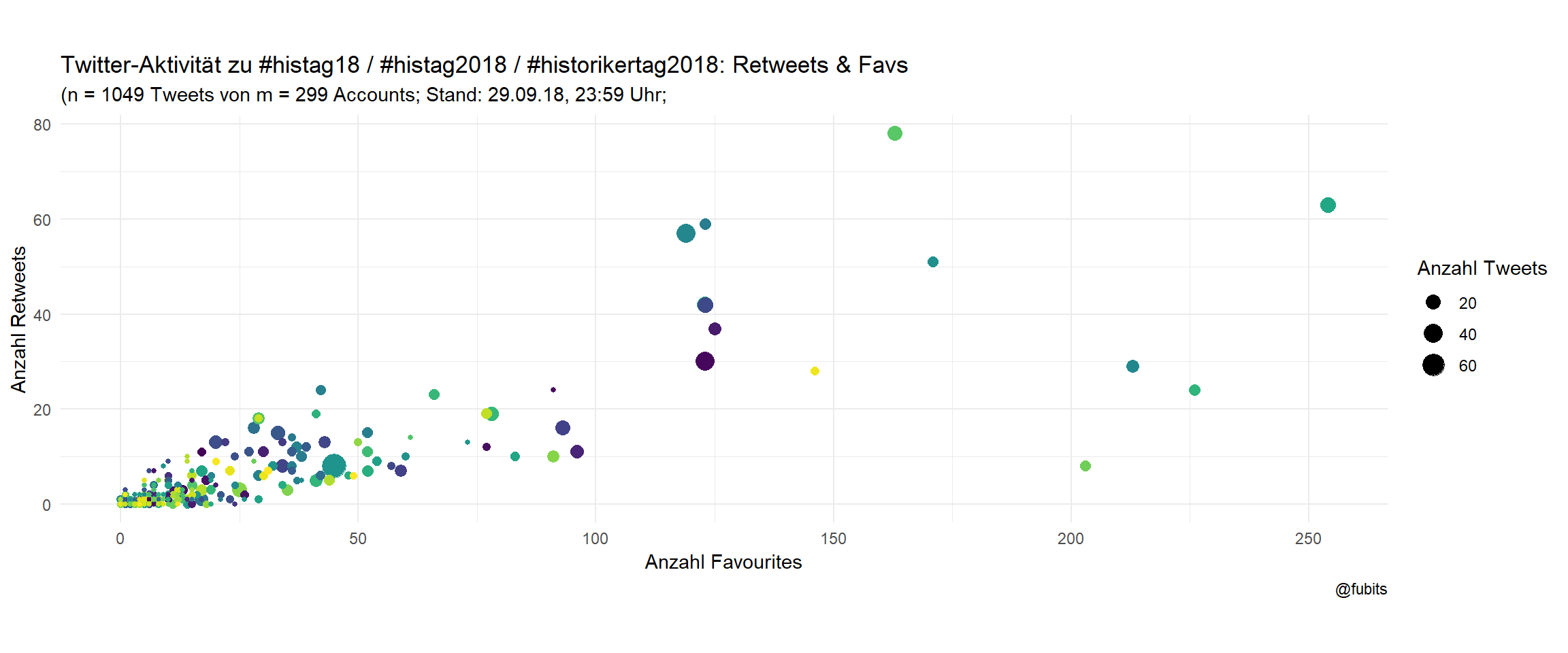
Historians: Top 20 labelled
ggplot(hist_counts, aes(x = Favs, y = RT)) +
    geom_point(aes(size = Tweets, color = screen_name), alpha = 0.5) +
    ggrepel::geom_text_repel(data = hist_counts[1:20,],
                             aes(label = screen_name)) +
    coord_fixed() +
    scale_color_viridis_d() +
    scale_x_continuous(breaks = scales::pretty_breaks(6)) +
    guides(color = FALSE) +
    theme_minimal() +
    labs(size = "Anzahl Tweets",
         title = "Twitter-Aktivität zu #histag18 / #histag2018 / #historikertag2018: Top 20 Accounts",
         subtitle = paste0("(n = ", hist_n_tweets,
                         " Tweets von m = ", hist_n_accounts,
                         " Accounts; Top 20 Label, Stand: 29.09.18, ",
                         "23:59", " Uhr)"),
         x = "Anzahl Favourites",
         y = "Anzahl Retweets",
         caption = "@fubits")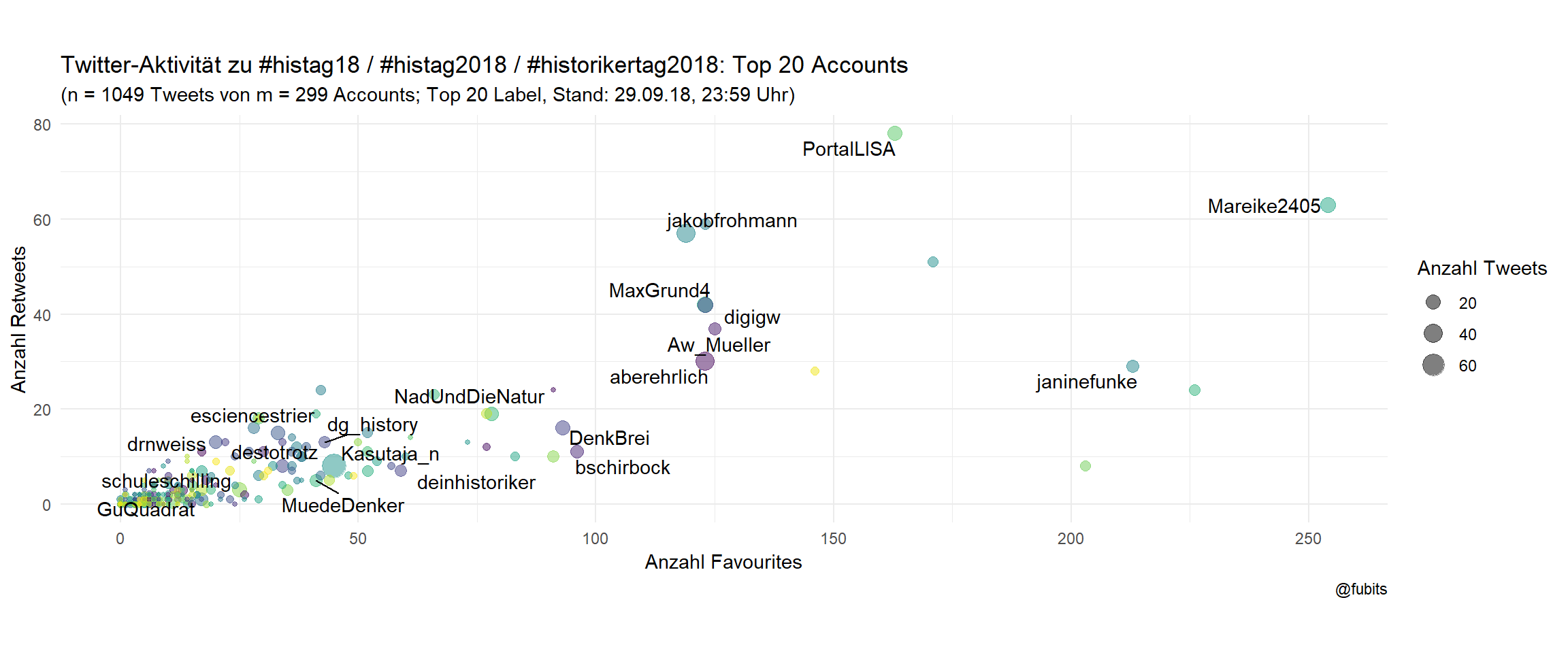
3.4 Computer Science: #informatik2018
(Of course, CS scholars are rather disciplined and stick to one hashtag :) #informatik18 has only 3 Tweets so far, and #informatiktage only 2 users…)
Mine
inf_tweets <- search_tweets(q = "#informatik2018", # explicit QUERY
      include_rts = FALSE,
      # max_id = ,
      n = 5000,
      verbose = TRUE,
      retryonratelimit = TRUE,
      type = "recent") # mixed recent popular

saveRDS(inf_tweets, file =
          str_c(data_path,"inf_tweets_",getTimeString(),".rds"))
Wrangle
inf_rds <- dir(path = data_path, pattern = "inf_") %>%
  str_c(data_path, .) %>%
  map_dfr(readRDS)
inf_collection <- inf_rds %>%
  distinct(status_id, .keep_all = TRUE) %>%
  filter(created_at > "2018-09-23" &
         created_at < "2018-09-30") %>%
  arrange(created_at)
Treemap
inf_n_tweets <- nrow(inf_collection)
inf_n_accounts <- length(unique(inf_collection$screen_name))

inf_collection %>%
  group_by(screen_name) %>%
  summarise(n = n()) %>%
  mutate(share = n / sum(n)) %>%
  arrange(desc(n)) %>%
  ggplot(aes(area = share)) +
    treemapify::geom_treemap(aes(fill = log10(n))) +
    treemapify::geom_treemap_text(
      aes(label = paste0(screen_name, " (", round(share*100,1),"%)"))
      ) +
  scale_fill_viridis_c(direction = -1, option = "C", begin = 0.8) +
  labs(title = "Twitter-Aktivität zu #informatik2018",
       subtitle = paste0("(n = ", inf_n_tweets,
                         " Tweets von m = ", inf_n_accounts,
                         " Accounts; Stand: 29.09.18, ",
                         "23:59" , " Uhr;",
                         " by @fubits)")) +
  guides(fill = FALSE)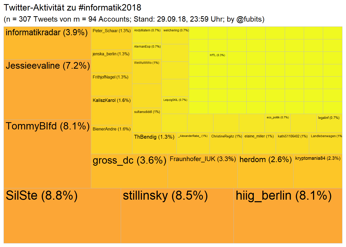
Hm, that’s quite a few Tweets for a presumably Tech-savie community…
Scatterplot with per-user activity
inf_counts <- inf_collection %>%
  group_by(screen_name) %>%
  # filter(screen_name != "fubits") %>%
  summarise(Tweets = n(),
            RT = sum(retweet_count),
            Favs = sum(favorite_count)) %>%
  mutate(discipline = "CS") %>%
  arrange(desc(Tweets))
  # top_n(n = 50, wt = tweets) %>%
ggplot(inf_counts, aes(x = Favs, y = RT)) +
geom_point(aes(size = Tweets, color = screen_name)) +
# ggrepel::geom_text_repel(data = counts[1:10,], aes(label = screen_name)) +
coord_fixed() +
scale_color_viridis_d() +
# scale_size_continuous(breaks = c(50, 100, 150, 200, 250, 300)) +
guides(color = FALSE) +
theme_minimal() +
labs(size = "Anzahl Tweets",
title = "Twitter-Aktivität zu #informatik2018: Retweets & Favs",
subtitle = paste0("(n = ", inf_n_tweets,
" Tweets von m = ", inf_n_accounts,
" Accounts; Stand: 29.09.18, ", "23:59" , " Uhr;"),
x = "Anzahl Favourites",
y = "Anzahl Retweets",
caption = "@fubits")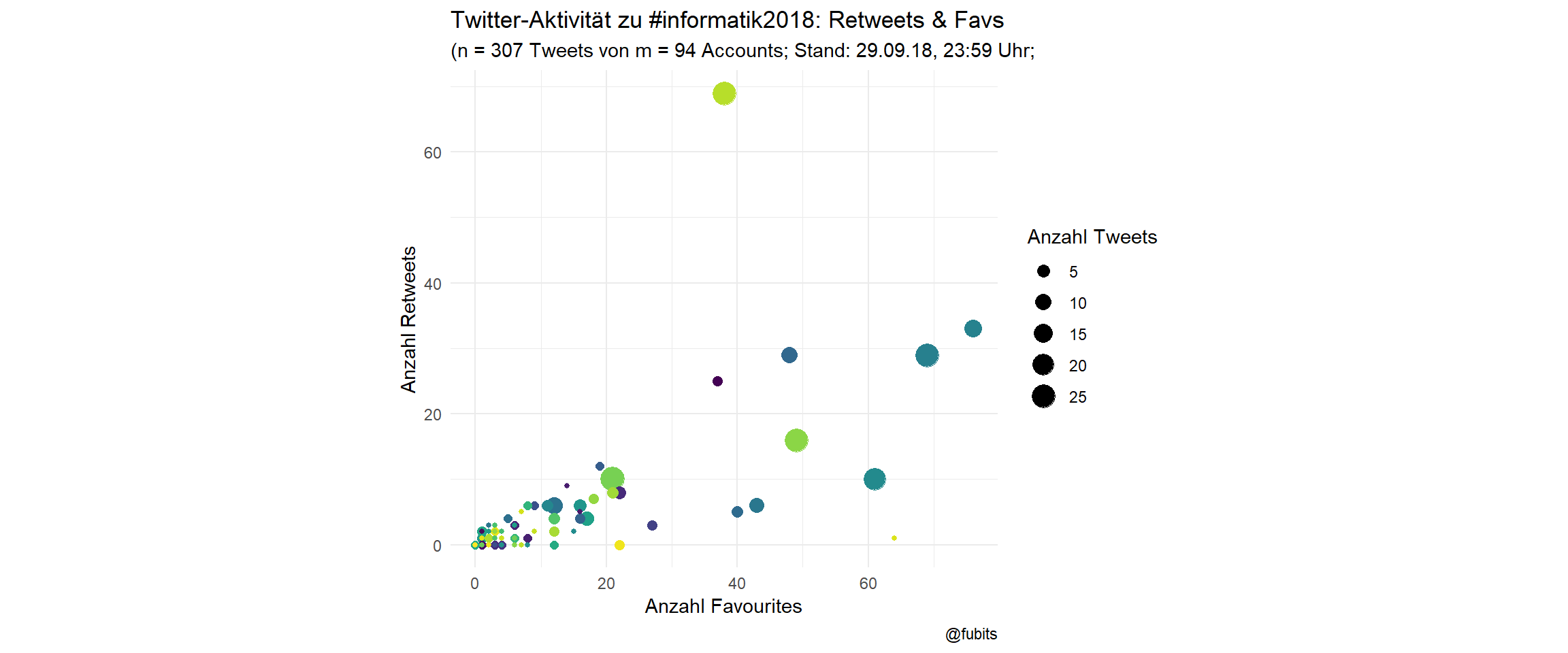
So there’s some truth in “I’m a Computer Scientist. We don’t use Twitter”…
Scatterplot: Top 20 labelled
ggplot(inf_counts, aes(x = Favs, y = RT)) +
    geom_point(aes(size = Tweets, color = screen_name), alpha = 0.5) +
    ggrepel::geom_text_repel(data = inf_counts[1:20,],
                             aes(label = screen_name)) +
    coord_fixed() +
    scale_color_viridis_d() +
    scale_x_continuous(breaks = c(0, 20, 40, 60, 80)) +
    guides(color = FALSE) +
    theme_minimal() +
    labs(size = "Anzahl Tweets",
         title = "Twitter-Aktivität zu #informatik2018: Top 20 Accounts",
         subtitle = paste0("(n = ", inf_n_tweets,
                         " Tweets von m = ", inf_n_accounts,
                         " Accounts; Top 20 Label, Stand: 29.09.18, ",
                         "23:59", " Uhr)"),
         x = "Anzahl Favourites",
         y = "Anzahl Retweets",
         caption = "@fubits")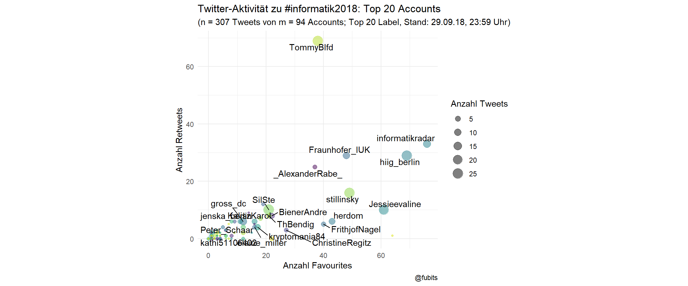
3.5 Media Studies: #gfm2018
As I have just been informed on Twitter, the German Society for Media Studies also had their annual meeting this week. That’s like some weird multidisciplinary but still strictly unidisciplinary academic conspiracy…
Nevertheless, let’s have a look at #gfm2018, too!
Mine
gfm_tweets <- search_tweets(q = "#gfm2018", # explicit QUERY
      include_rts = FALSE,
      # max_id = ,
      n = 5000,
      verbose = TRUE,
      retryonratelimit = TRUE,
      type = "recent") # mixed recent popular

saveRDS(gfm_tweets, file =
          str_c(data_path,"gfm_tweets_",getTimeString(),".rds"))
Wrangle
gfm_rds <- dir(path = data_path, pattern = "gfm_") %>%
  str_c(data_path, .) %>%
  map_dfr(readRDS)
gfm_collection <- gfm_rds %>%
  distinct(status_id, .keep_all = TRUE) %>%
  filter(created_at > "2018-09-23" &
         created_at < "2018-09-30") %>%
  arrange(created_at)
Treemap
gfm_n_tweets <- nrow(gfm_collection)
gfm_n_accounts <- length(unique(gfm_collection$screen_name))

gfm_collection %>%
  group_by(screen_name) %>%
  summarise(n = n()) %>%
  mutate(share = n / sum(n)) %>%
  arrange(desc(n)) %>%
  ggplot(aes(area = share)) +
    treemapify::geom_treemap(aes(fill = log10(n))) +
    treemapify::geom_treemap_text(
      aes(label = paste0(screen_name, " (", round(share*100,1),"%)"))
      ) +
  scale_fill_viridis_c(direction = -1, option = "C", begin = 0.8) +
  labs(title = "Twitter-Aktivität zu #gfm2018",
       subtitle = paste0("(n = ", gfm_n_tweets,
                         " Tweets von m = ", gfm_n_accounts,
                         " Accounts; Stand: 29.09.18, ",
                         "23:59" , " Uhr;",
                         " by @fubits)")) +
  guides(fill = FALSE)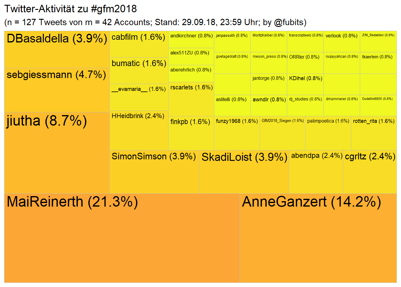
Let’s treat this as preliminary. I’ve just mined the Tweets for the first time, so a couple more samples might another couple of Tweets. Don’t expect the numbers to double, though!
Scatterplot with per-user activity
gfm_counts <- gfm_collection %>%
  group_by(screen_name) %>%
  # filter(screen_name != "fubits") %>%
  summarise(Tweets = n(),
            RT = sum(retweet_count),
            Favs = sum(favorite_count)) %>%
  mutate(discipline = "MediaStudies") %>%
  arrange(desc(Tweets))
  # top_n(n = 50, wt = tweets) %>%
Since there’s not too much activity for #gfm2018, we can jump to the labelled scatterplot.
Scatterplot: Top 20 labelled
ggplot(gfm_counts, aes(x = Favs, y = RT)) +
    geom_point(aes(size = Tweets, color = screen_name), alpha = 0.5) +
    ggrepel::geom_text_repel(data = gfm_counts[1:20,],
                             aes(label = screen_name)) +
    coord_fixed() +
    scale_color_viridis_d() +
    scale_x_continuous(breaks = c(0, 10, 20, 40, 50, 110)) +
    guides(color = FALSE) +
    theme_minimal() +
    labs(size = "Anzahl Tweets",
         title = "Twitter-Aktivität zu #gfm2018: Top 20 Accounts",
         subtitle = paste0("(n = ", gfm_n_tweets,
                         " Tweets von m = ", gfm_n_accounts,
                         " Accounts; Top 20 Label, Stand: 29.09.18, ",
                         "23:59", " Uhr)"),
         x = "Anzahl Favourites",
         y = "Anzahl Retweets",
         caption = "@fubits")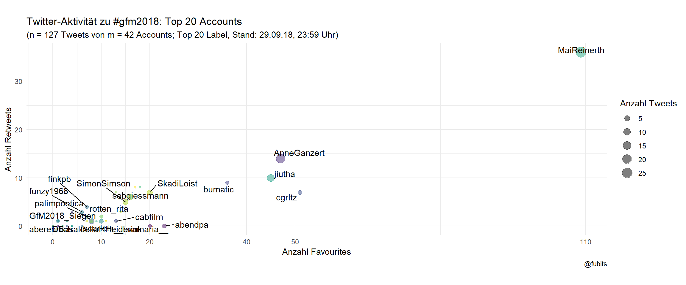
4 Some Comparisons
Now, we will need to bind the four tibbles together. First, let’s get the total numbers of unique Tweets and unique users:
all_cons <- bind_rows(dvpw_collection, dgs_collection, hist_collection, inf_collection, gfm_collection)
all_n_accounts <- all_cons %>% distinct(screen_name) %>% nrow()
all_n_tweets <- all_cons %>% distinct(status_id) %>% nrow()
So, this week, 751 German academic Twitter accounts have been active at four five conferences in total, producing 3815 individual Tweets. Actually, that’s quite impressive!
Now we can bind the aggregated *_counts.
all_cons_per_user <- bind_rows(dvpw_counts, dgs_counts, hist_counts, inf_counts, gfm_counts) %>%
  group_by(screen_name) %>%
  distinct(screen_name, .keep_all = TRUE) %>%
  mutate(avg_output = (Tweets + RT + Favs)/3) %>%
  arrange(desc(avg_output)) #> 1262
# all_cons_per_user %>% distinct(screen_name) %>% count() #> 1262
all_cons_per_user %>% head(20) %>% knitr::kable("html", digits = 2)| screen_name | Tweets | RT | Favs | discipline | avg_output |
|---|---|---|---|---|---|
| dvpw | 460 | 496 | 580 | PolSci | 512.00 |
| dvpwkongress | 123 | 160 | 311 | PolSci | 198.00 |
| thothiel | 43 | 81 | 249 | PolSci | 124.33 |
| Mareike2405 | 23 | 63 | 254 | History | 113.33 |
| ronpatz | 56 | 59 | 204 | PolSci | 106.33 |
| PortalLISA | 20 | 78 | 163 | History | 87.00 |
| moritz_hoffmann | 9 | 24 | 226 | History | 86.33 |
| janinefunke | 12 | 29 | 213 | History | 84.67 |
| SassanGholiagha | 85 | 30 | 131 | PolSci | 82.00 |
| elvira_rosert | 40 | 41 | 164 | PolSci | 81.67 |
| LordElend | 26 | 32 | 184 | Sociology | 80.67 |
| juergenzimmerer | 7 | 51 | 171 | History | 76.33 |
| RichterHedwig | 7 | 8 | 203 | History | 72.67 |
| DrMichaelHein | 20 | 29 | 168 | PolSci | 72.33 |
| jakobfrohmann | 38 | 57 | 119 | History | 71.33 |
| wahlforschung | 34 | 35 | 144 | PolSci | 71.00 |
| PetraGuasti | 84 | 28 | 92 | PolSci | 68.00 |
| daniellambach | 33 | 38 | 133 | PolSci | 68.00 |
| aberehrlich | 40 | 30 | 123 | History | 64.33 |
| MaxGrund4 | 26 | 42 | 123 | History | 63.67 |
4.1 Joint Scatterplot: per-User
Let’s have a look at this week’s German academic Twitter crowd as a whole:
ggplot(all_cons_per_user,
       aes(x = Favs, y = RT, color = fct_inorder(discipline))) +
    geom_point(aes(size = Tweets), alpha = 0.5) +
    ggrepel::geom_text_repel(data = all_cons_per_user[1,],
                             aes(label = screen_name)) +
    coord_fixed() +
    scale_color_viridis_d(option = "D") +
    scale_x_continuous(breaks = c(0, 100, 200, 300, 400)) +
    theme_minimal() +
    guides(color = guide_legend(override.aes = list(size = 5,
                                                    stroke = 1.5)
                                )) +
    labs(size = "Anzahl Tweets",
         color = "Disziplin",
         title = "Twitter-Aktivität zu Twitter-Aktivität zu #dvpw*18, #dgs*18, #hist*18, #informatik2018 und #gfm2018: Top 20 Accounts",
         subtitle = paste0("(n = ", all_n_tweets,
                         " Tweets von m = ", all_n_accounts,
                         " Accounts; Top 20 Label, Stand: 29.09.18, ",
                         "23:59", " Uhr)"),
         x = "Anzahl Favourites",
         y = "Anzahl Retweets",
         caption = "@fubits")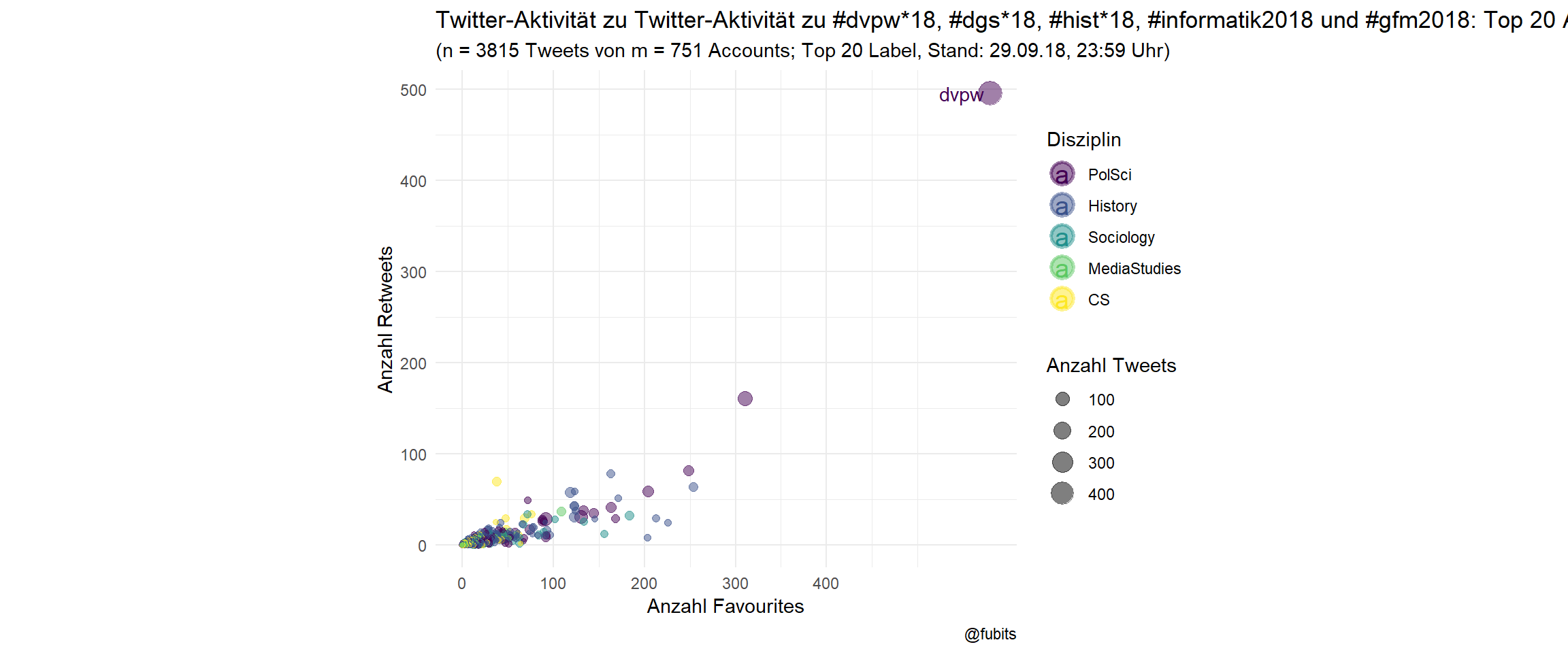
4.2 Joint Scatterplot: Top 20 labelled (w/o @dvpw)
all_cons_per_user %>%
  filter(screen_name != "dvpw") %>%
  ggplot(aes(x = Favs, y = RT, color = fct_inorder(discipline))) +
    geom_point(aes(size = Tweets), alpha = 0.5) +
    ggrepel::geom_text_repel(data = all_cons_per_user[2:21,],
                             aes(label = screen_name), alpha = 1) +
    coord_fixed() +
    scale_color_viridis_d(option = "D") +
    scale_x_continuous(breaks = scales::pretty_breaks()) +
    theme_minimal() +
    guides(colour = guide_legend(override.aes = list(size = 5,
                                                     stroke = 1.5)
                                 )) +
    labs(size = "Anzahl Tweets",
         color = "Disziplin",
         title = "Twitter-Aktivität zu #dvpw*18, #dgs*18, #hist*18, #informatik2018 und #gfm2018: Top 20 Accounts",
         subtitle = paste0("(n = ",
                           sum(filter(all_cons_per_user,
                                      screen_name != "dvpw")$Tweets),
                         " Tweets von m = ", all_n_accounts-1,
                         " Accounts (ohne @dvpw); Top 20 Label, Stand: 29.09.18, ","23:59", " Uhr)"),
         x = "Anzahl Favourites",
         y = "Anzahl Retweets",
         caption = "@fubits")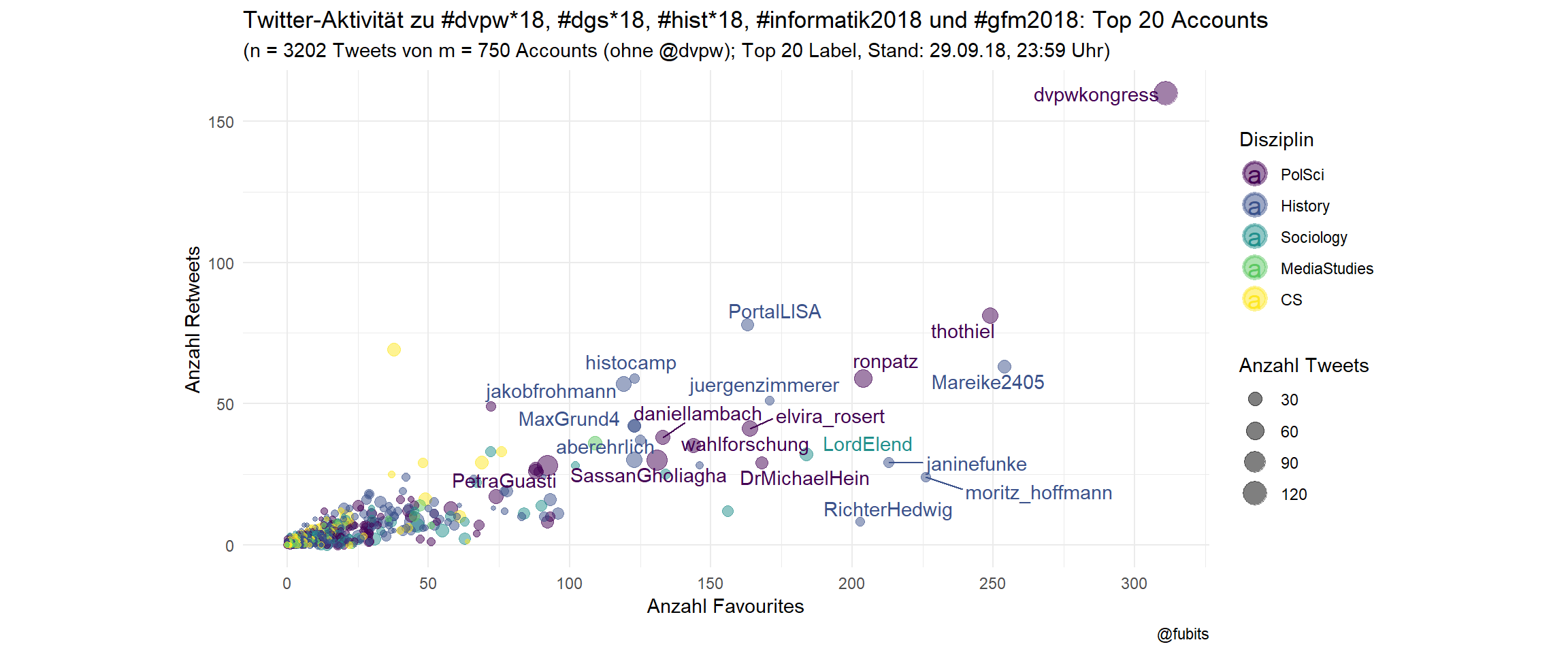
That’s what one week of academic twitter activity in Germany looks like, Duh!
4.3 Boxplots: Overall Distribution of Activities by Discipline
For Boxplot, we need to wrangle the data into long (~tidy) form:
dvpw_box <- dvpw_counts %>%
  gather("Metric", "Total", 2:4) #%>%
  # mutate(Discipline = "PolSci")
dvpw_box %>% filter(screen_name == "dvpw") %>% knitr::kable(format = "html")| screen_name | discipline | Metric | Total |
|---|---|---|---|
| dvpw | PolSci | Tweets | 460 |
| dvpw | PolSci | RT | 496 |
| dvpw | PolSci | Favs | 580 |
dgs_box <- dgs_counts %>%
  gather("Metric", "Total", 2:4) # %>%
  # mutate(Discipline = "Socio")

hist_box <- hist_counts %>%
  gather("Metric", "Total", 2:4) # %>%
  # mutate(Discipline = "History")

inf_box <- inf_counts %>%
  gather("Metric", "Total", 2:4) # %>%
  # mutate(Discipline = "CS")

gfm_box <- gfm_counts %>%
  gather("Metric", "Total", 2:4) # %>%
  # mutate(Discipline = "CS")
bind_rows(dvpw_box, dgs_box, hist_box, inf_box, gfm_box) %>%
ggplot() +
geom_boxplot(aes(fct_inorder(Metric), Total)) +
scale_x_discrete() +
scale_fill_viridis_d() +
facet_wrap(vars(discipline)) +
theme_light()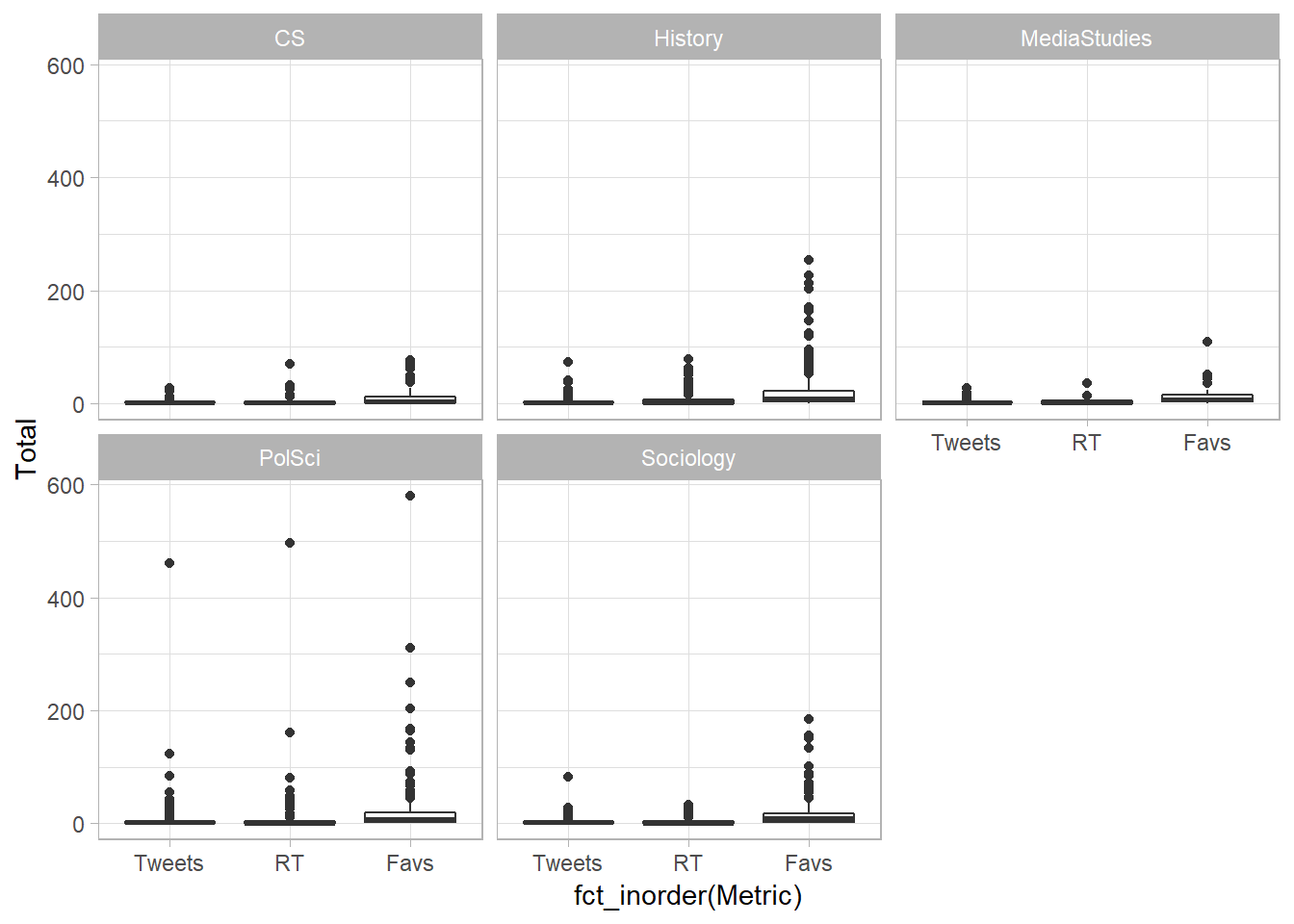
Hm, maybe Violin Plots can reveal more?
bind_rows(dvpw_box, dgs_box, hist_box, inf_box, gfm_box) %>%
  ggplot() +
  geom_violin(aes(fct_inorder(Metric), Total, fill = Metric)) +
  scale_x_discrete() +
  scale_fill_viridis_d() +
  facet_wrap(vars(discipline)) +
  labs(x = "Distribution of Tweets / RT / Favs per User",
       legend = NULL) +
  theme_light()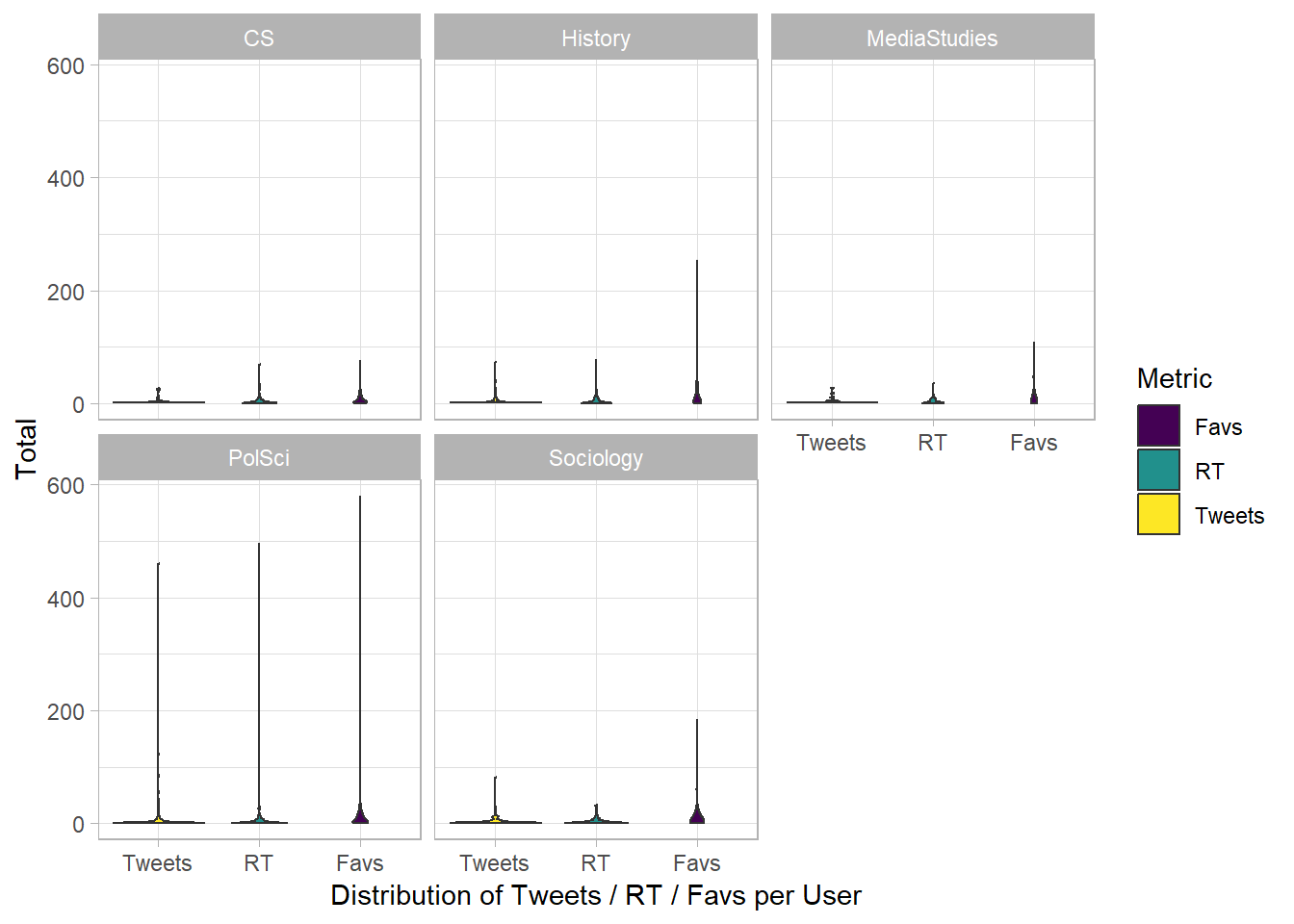
Mmmh, ok, I think I should try those beeswarm-plots soon-ish here…
5 Final scores: The overall activity compared by numbers
What if we simply compare the five disciplines’ Twitter performance in terms of totals?
bind_rows(dvpw_counts, dgs_counts, hist_counts, inf_counts, gfm_counts) %>%
  group_by(discipline) %>%
  summarise(Users = n(), Tweets = sum(Tweets),
            RT = sum(RT), Fav = sum(Favs)) %>%
  arrange(desc(Users)) %>%
knitr::kable(format = "html", digits = 2)| discipline | Users | Tweets | RT | Fav |
|---|---|---|---|---|
| History | 299 | 1049 | 1514 | 6362 |
| PolSci | 240 | 1752 | 1678 | 5203 |
| Sociology | 150 | 641 | 514 | 2677 |
| CS | 94 | 307 | 394 | 1020 |
| MediaStudies | 42 | 127 | 147 | 582 |
Sociology History has the highest number of active users and Favs (wow!), while PolSci has a lead with the total number of Tweets.
And what if we average out Tweets+RTs+Favs per User?
bind_rows(dvpw_counts, dgs_counts, hist_counts, inf_counts, gfm_counts) %>%
  group_by(discipline) %>%
  summarise(Users = n(), Tweets = sum(Tweets),
            RT = sum(RT), Fav = sum(Favs)) %>%
  mutate(avg_output = (Tweets + RT + Fav) / Users) %>%
  arrange(desc(avg_output)) %>%
knitr::kable(format = "html", digits = 2)| discipline | Users | Tweets | RT | Fav | avg_output |
|---|---|---|---|---|---|
| PolSci | 240 | 1752 | 1678 | 5203 | 35.97 |
| History | 299 | 1049 | 1514 | 6362 | 29.85 |
| Sociology | 150 | 641 | 514 | 2677 | 25.55 |
| MediaStudies | 42 | 127 | 147 | 582 | 20.38 |
| CS | 94 | 307 | 394 | 1020 | 18.31 |
Here, the PolSci crowd has been the busiest (and Sociology was rather lazy). But…
... let’s have look without the #TeamTakeOver coup by @dvpw:
bind_rows(dvpw_counts, dgs_counts, hist_counts, inf_counts, gfm_counts) %>%
  filter(screen_name != "dvpw") %>%
  group_by(discipline) %>%
  summarise(Users = n(), Tweets = sum(Tweets),
            RT = sum(RT), Fav = sum(Favs)) %>%
  mutate(avg_output = (Tweets + RT + Fav) / Users) %>%
  arrange(desc(avg_output)) %>%
knitr::kable(format = "html", digits = 2)| discipline | Users | Tweets | RT | Fav | avg_output |
|---|---|---|---|---|---|
| History | 299 | 1049 | 1514 | 6362 | 29.85 |
| PolSci | 239 | 1292 | 1182 | 4623 | 29.69 |
| Sociology | 150 | 641 | 514 | 2677 | 25.55 |
| MediaStudies | 42 | 127 | 147 | 582 | 20.38 |
| CS | 94 | 307 | 394 | 1020 | 18.31 |
Well done, Historians! If we ignore @dvpw’s Twitter takeover, you actually performed best (in terms of numbers, at least)!
I guess it is fair to conclude that a well organised Twitter takeover by conference participants can have quite an effect on the visibility of a conference.
Further interpretation is up to you :)
6 What’s next?
One hint:
library(quanteda)
library(tidygraph)
But that is for another post…