[R] German Academic Twitter, Pt. 2: From Data to Corpus with a Turkish Twist
Abstract / TL;DR
We'll learn about constructing a document-feature matrix (dfm), applying exhaustive stopword-lists, the pitfalls of working with text as data, and most importantly acknowledge and learn from mistakes...
Last week, I mined almost 5K Tweets from the annual meetings of five German academic societies. Now it’s about time that we dive into the contents with Kenneth Benoit’s powerful quanteda Package. Come for the corpus approaches to text as data, stay for the Turkish Plot-Twist…
library(tidyverse)
library(here)
library(rtweet) # just in case we want to look up something on Twitter
library(quanteda)
quanteda_options("threads" = 4)
# quanteda_options("threads")
1 Import Tweets from .rds
Please see Twitter pt. 1 for Twitter Mining with rtweet and the details of the data handling approach.
Prepare here()-path to the .rds data
data_path <- here("data", "ConferenceTweets", "/")Bulk-read the .rds files
dvpw_collection <- dir(path = data_path, pattern = "dvpw_") %>%
  str_c(data_path, .) %>%
  map_dfr(readRDS)
dvpw_collection <- dvpw_collection %>% distinct(status_id, .keep_all = TRUE) %>%
  filter(created_at < "2018-09-30") %>%
  mutate(Discipline = "PolSci") %>%
  arrange(created_at)

dgs_collection <- dir(path = data_path, pattern = "dgs_") %>%
  str_c(data_path, .) %>%
  map_dfr(readRDS)
dgs_collection <- dgs_collection %>% distinct(status_id, .keep_all = TRUE) %>%
  filter(created_at < "2018-09-30") %>%
  mutate(Discipline = "Sociology") %>%
  arrange(created_at)

hist_collection <- dir(path = data_path, pattern = "hist_") %>%
  str_c(data_path, .) %>%
  map_dfr(readRDS)
hist_collection <- hist_collection %>% distinct(status_id, .keep_all = TRUE) %>%
  filter(created_at < "2018-09-30") %>%
  mutate(Discipline = "History") %>%
  arrange(created_at)

inf_collection <- dir(path = data_path, pattern = "inf_") %>%
  str_c(data_path, .) %>%
  map_dfr(readRDS)
inf_collection <- inf_collection %>% distinct(status_id, .keep_all = TRUE) %>%
  filter(created_at < "2018-09-30") %>%
  mutate(Discipline = "CS") %>%
  arrange(created_at)
1.1 Subset “Interdisciplinary” Tweets
Something I didn’t account for last time, was the possibility that some Twitter Users might have been mentioning / monitoring multiple conferences, esp. with regards to the interrelation between Political Science, Sociology, and History.
Let’s single them out and assign a “Mixed” label.
joint_collection <- bind_rows(dvpw_collection, dgs_collection,
                              hist_collection, inf_collection)

# build set of distinct
joint_distinct <- joint_collection %>%
  distinct(status_id, .keep_all = TRUE)

#subset duplicated
mixed_collection <- subset(joint_collection,
                      duplicated(joint_collection$status_id)) %>%
  distinct(status_id, .keep_all = TRUE) # find duplicates

mixed_collection$Discipline <- "Mixed"
Only 42 Tweets? Out of a sample of almost 5K? Twitter Silos, anyone?
1.2 Inspect “Interdisciplinary” Tweets
mixed_collection %>%
  arrange(created_at) %>%
  select(text) %>% head(10) %>%
knitr::kable(format = "html", digits = 2)| text |
|---|
| Gut, dass das Team des @fgf_nrw etwas größer ist: Wir sind diese Woche vertreten: #dgs18, #dvpw18 und ab Mittwoch bei der KEG in Wien https://t.co/jiE6SyfKHe |
| Hier noch eine wichtige Ansage: #dvpw18 muss unbedingt vor #dgs18 trenden |
| @daniellambach Das wollen die von den Naturwissenschaften doch nur, dass wir Sozial- und Geisteswissenschaftler*innen uns gegenseitig bekriegen. 😉 #dvpw18 #histag18 #dgs18 |
| Leider findet die #dvpw18 gleichzeitig mit dem #dgs2018 statt. Wäre sehr gern auch bei Euch, @mlewandowsky, @wahlforschung und @thothiel :/ |
| Paar Minuten im 1. Vortrag #infdh2018 reichen schon, um mal ganz deutlich zu sehen um wie viele Größenordnungen die digitalen Geisteswissenschaften den “digitalen” Sozialwissenschaften handwerklich und institutionell voraus sind. Grüße an #dvpw18 und #dgs18 https://t.co/TZU8E9PecT |
| Meine Wunsch an #ScienceTwitter jetzt wo #dvpw18 & #HisTag18 & #dgs18 parallel laufen: Kann jemand analysieren, wie viel Schnittmenge es zwischen den Programmen gibt? |
| @DrMichaelHein @dvpwkongress #dgs18 #dvpw18 #histag18 ich fände es ja schöner auf spannende Themen gemeinsam zu blicken, die wir gesellschaftlich gemeinsam diskutieren könnten/sollten, und nicht Trennungslinien und Wettbewerb aufzumachen… |
| Kleine Pause gefällig? Unter den Hashtags #ddss18, #dgs18 und #HisTag18 kann man sehr interessanten Veranstaltungen aus der Ferne beiwohnen. #gswtud https://t.co/VlfzaYpjrb |
| Wie wäre es mit einem gemeinsamen Soziohistostaatsrechtspolitolog*innentag 2021? @dvpwkongress @dvpw @DGSoziologie @historikertag @vdstrl #dvpw18 #histag18 #dgs18 #vdstrl18 https://t.co/EgZYmaikqY |
| während die lieben kolleg(inn)en bei #dvpw18, #dgs18 & #HisTag18 um die besten tweets auf #twitter ringen, schauen wir von #GSA2018 aus pittsburgh zu. good luck, friends! 😇 |
2 Create Corpus
For further, “Corpus-based”" analysis (and beyond) we’ll use the quanteda package.
I aim to re-do as much as I can from this series with Julia Silge’s tidytext package, soon, btw.
2.1 Build Individual Corpora
As we already have singled out “interdisciplinary” Tweets, we’ll just anti_join() every other tibble with the mixed Tweets.
dvpw_corpus <- dvpw_collection %>%
  anti_join(mixed_collection, by = "status_id") %>%
  corpus(docid_field = "status_id")
docvars(dvpw_corpus, "Discipline") <- "PolSci"

dgs_corpus <- dgs_collection %>%
  anti_join(mixed_collection, by = "status_id") %>%
  corpus(docid_field = "status_id")
docvars(dgs_corpus, "Discipline") <- "Sociology"

hist_corpus <- hist_collection %>%
  anti_join(mixed_collection, by = "status_id") %>%
  corpus(docid_field = "status_id")
docvars(hist_corpus, "Discipline") <- "History"

inf_corpus <- inf_collection %>%
  anti_join(mixed_collection, by = "status_id") %>%
  corpus(docid_field = "status_id")
docvars(inf_corpus, "Discipline") <- "CS"

mixed_corpus <- mixed_collection  %>%
  corpus(docid_field = "status_id")
docvars(mixed_corpus, "Discipline") <- "Mixed"
2.2 Create Joint Corpus
That’s even easier thanks to Quanteda.
joint_corpus <- dvpw_corpus +
                dgs_corpus +
                hist_corpus +
                inf_corpus +
                mixed_corpus
3 Create DFM
For most really usuful approaches to “text as data” we’ll need a sparse document-feature matrix (dfm). Doing this with quanteda is straight forward, but there are some less prominent Tweets.
3.1 Naive
joint_dfm <- dfm(joint_corpus,
                # groups = "Discipline",
                 remove_punct = TRUE,
                 remove_url = TRUE, # it's a mess, without
                 tolower = TRUE,
                 verbose = FALSE) #for website readability
topfeatures(joint_dfm, 20) %>%
knitr::kable(format = "html", digits = 2)| x | |
|---|---|
| der | 2001 |
| #dvpw18 | 1681 |
| und | 1661 |
| die | 1517 |
| in | 1214 |
| #dgs2018 | 1174 |
| #histag18 | 1037 |
| auf | 765 |
| von | 675 |
| für | 624 |
| zu | 601 |
| #dgs18 | 584 |
| das | 583 |
| mit | 566 |
| ist | 520 |
| the | 515 |
| den | 480 |
| des | 452 |
| im | 437 |
| dem | 432 |
We get nfeat(joint_dfm) = 20832 features, but as we can see from the topfeatures() output, the top features are mostly (and unsurprisingly very common German words which are also know as stopwords in NLP).
3.2 2nd Attempt: Remove stopwords("german")
joint_dfm <- dfm(joint_corpus,
# groups = "Discipline",
remove = stopwords("german"),
remove_punct = TRUE,
remove_url = TRUE,
tolower = TRUE,
verbose = FALSE)
topfeatures(joint_dfm, 20) %>%
knitr::kable(format = "html", digits = 2)| x | |
|---|---|
| #dvpw18 | 1681 |
| #dgs2018 | 1174 |
| #histag18 | 1037 |
| #dgs18 | 584 |
| the | 515 |
| of | 357 |
| and | 337 |
| #informatik2018 | 321 |
| to | 314 |
| amp | 224 |
| a | 223 |
| heute | 200 |
| beim | 184 |
| on | 175 |
| panel | 172 |
| dass | 168 |
| @dvpwkongress | 166 |
| for | 162 |
| is | 150 |
| demokratie | 145 |
Apart from English tokens (to, on, is, for, of, a), common German words such as “beim” or “dass” are still included. The latter is rather weird…
3.2.1 Inspect quanteda's built-in Stop Words
Since we’ve seen that “dass” is still included in our corpus, let’s i.e. look at all quanteda::stopwords("german") starting with a “d”:
stopwords("german") %>%
  as_tibble() %>%
  filter(str_detect(value, pattern = "^da.*")) %>%
knitr::kable(format = "html", digits = 2)| value |
|---|
| da |
| damit |
| dann |
| das |
| daß |
| dasselbe |
| dazu |
Ok, “beim” is missing, and “daß” instead of “dass” suggests that
quanteda’s German stopword list terms might need an update… :)
Also, note how stopwords("german") consists of 231 tokens. Just for comparison, tidytext::stop_words has a total of 1149 stopwords for English. So we probably will have to include custom stopword lists repeatedly.
Of course, GitHub has you covered! Gene Diaz is maintaining a super-exhaustive list of stopwords for multiple languages: github.com/stopwords-iso
We’ll use the text file with the German stopwords: stopwords-de.txt
ger_stopwords <- read_lines("https://raw.githubusercontent.com/stopwords-iso/stopwords-de/master/stopwords-de.txt")
# saveRDS(ger_stopwords, "ger_stopwords.rds")
length(ger_stopwords) #> 621 stopwords
c(ger_stopwords, stopwords("german")) %>% length() #> 852
c(ger_stopwords, stopwords("german")) %>% unique() %>% length() #> 6213.2.2 Include Custom Stopwords and Remove English Stopwords
c("dass", "beim") %in% ger_stopwords #> [1] TRUE TRUE## [1] TRUE TRUE# custom_stopwords <- c("dass", "beim")
custom_stopwords <- setdiff(ger_stopwords, stopwords("german")) # only keep left setjoint_dfm <- dfm(joint_corpus,
# groups = "Discipline",
remove = c(stopwords("german"),
stopwords("english"), # ONE
custom_stopwords, # TWO
min_nchar = 2), # THREE
remove_punct = TRUE,
remove_url = TRUE,
tolower = TRUE,
verbose = FALSE)
topfeatures(joint_dfm, 20) %>%
knitr::kable(format = "html", digits = 2)| x | |
|---|---|
| #dvpw18 | 1681 |
| #dgs2018 | 1174 |
| #histag18 | 1037 |
| #dgs18 | 584 |
| #informatik2018 | 321 |
| amp | 224 |
| panel | 172 |
| @dvpwkongress | 166 |
| demokratie | 145 |
| @osymbaskanligi | 123 |
| dgs | 121 |
| innen | 114 |
| #dgs | 113 |
| @dvpw | 112 |
| #dvpw2018 | 111 |
| @historikertag | 109 |
| bu | 106 |
| de | 97 |
| @dgsoziologie | 95 |
| mı | 94 |
Great. But … what is “amp”???
3.2.3 Inspect “Keyword in Context” kwic() for “amp”
kwic(joint_corpus, "amp", window = 3)  %>%
  # vs. kwic(x, phrase("term1 term2"))
  as_tibble() %>% # needed for kwic()
  select(pre:post) %>%
  head(10) %>%
knitr::kable(format = "html", digits = 2)| pre | keyword | post |
|---|---|---|
| @ifp_tuebingen ) & | amp | ; I organise |
| @goetheuni ) & | amp | ; Jonas Wolff |
| public goods & | amp | ; to prevent |
| die Vorträge & | amp | ; Panelleitungen von |
| von #InIIS & | amp | ; @BIGSSS_Bremen Kolleg |
| Viel Erfolg & | amp | ; Spaß den |
| " #PolComm & | amp | ; Digital Complexity |
| , @SFB1342 & | amp | ; von überall |
| bestimmt spannende & | amp | ; inspirierende Tage |
| nach #Adorno & | amp | ; Co gehen |
“amp” == “&” which is the
HTMLterm for & / ampersand (but “&” is removed when we create the corpus withremove_punct = TRUE, so only “amp” remains. Cool.)
Remove “amp”
custom_stopwords <- c(custom_stopwords, "amp")
# This way, we'll keep our custom "amp" and "innen"
joint_dfm <- dfm(joint_corpus,
                 # groups = "Discipline",
                 remove = c(stopwords("german"),
                            stopwords("english"),
                            custom_stopwords,
                            min_nchar = 2),
                 remove_punct = TRUE,
                 remove_url = TRUE,
                 tolower = TRUE,
                 verbose = FALSE)
topfeatures(joint_dfm, 20) %>%
knitr::kable(format = "html", digits = 2)| x | |
|---|---|
| #dvpw18 | 1681 |
| #dgs2018 | 1174 |
| #histag18 | 1037 |
| #dgs18 | 584 |
| #informatik2018 | 321 |
| panel | 172 |
| @dvpwkongress | 166 |
| demokratie | 145 |
| @osymbaskanligi | 123 |
| dgs | 121 |
| innen | 114 |
| #dgs | 113 |
| @dvpw | 112 |
| #dvpw2018 | 111 |
| @historikertag | 109 |
| bu | 106 |
| de | 97 |
| @dgsoziologie | 95 |
| mı | 94 |
| thema | 93 |
That’s better. But what’s up with “innen” and “bu”?
3.2.4 Inspect the Tokens "innen" and "bu" kwic().
kwic(joint_corpus, "innen", window = 3)  %>%
  as_tibble() %>% # needed for kwic()
  select(pre:post) %>%
  head(10) %>%
knitr::kable(format = "html", digits = 2)| pre | keyword | post |
|---|---|---|
| @BIGSSS_Bremen Kolleg * | innen | . Da ist |
| | ler * | innen | vor Ort #powi |
| #powi Kolleg * | innen | von @UniBremen , |
| . Kolleg / | innen | der @unihh im |
| Kolleg / | innen | vom Institut für |
| die Kolleg / | innen | mit dem Peer |
| 1000 Expert * | innen | sucht , die |
| loyale Bürger / | innen | oder auch bürgerliche |
| mit Rassist * | innen | , Antisemit * |
| , Antisemit * | innen | , und Nazis |
Ok, so
"< / | * >innen"is part of the gendered forms of plurals of German terms such as Colleagues, Citizens, Rassists et al. We might want to think of a robust solution - which should not be stemming - here. Maybengrams=2or some cleverstr_c(<regex> + (* | /) + "innen"")might help. But for now we’ll just add"innen"as a stopword.
custom_stopwords <- c(custom_stopwords, "innen")
joint_dfm <- dfm(joint_corpus,
                 # groups = "Discipline",
                 remove = c(stopwords("german"),
                            stopwords("english"),
                            custom_stopwords,
                            min_nchar = 2),
                 remove_punct = TRUE,
                 remove_url = TRUE,
                 tolower = TRUE,
                 verbose = FALSE)
topfeatures(joint_dfm, 20) %>%
knitr::kable(format = "html", digits = 2)| x | |
|---|---|
| #dvpw18 | 1681 |
| #dgs2018 | 1174 |
| #histag18 | 1037 |
| #dgs18 | 584 |
| #informatik2018 | 321 |
| panel | 172 |
| @dvpwkongress | 166 |
| demokratie | 145 |
| @osymbaskanligi | 123 |
| dgs | 121 |
| #dgs | 113 |
| @dvpw | 112 |
| #dvpw2018 | 111 |
| @historikertag | 109 |
| bu | 106 |
| de | 97 |
| @dgsoziologie | 95 |
| mı | 94 |
| thema | 93 |
| bir | 89 |
4 The Turkish Plot-Twist
4.1 One last Mystery remains…
So what about "bu"?
(Spoiler:
@osymbaskanligiseems to be an offical governmental Turkish account… That already points at something bigger.)
kwic(joint_corpus, "bu", window = 3) %>%
  as_tibble() %>% # needed for kwic()
  select(pre:post) %>%
  head(10) %>%
knitr::kable(format = "html", digits = 2)| pre | keyword | post |
|---|---|---|
| #dgs2018 keşke | bu | gece açıklansa 🙄 |
| #dgs2018 | bu | gecenin en büyük |
| otomatik olarak yapıyorsa | bu | bekleyiş neden ? |
| sonuçlarını açıklamak neden | bu | kadar uzun sürüyor |
| Bu | yaşta bu kadar | |
| Bu yaşta | bu | kadar sıkıntı yeter |
| @OSYMbaskanligi ceza mı | bu | ne şimdi #dgs2018 |
| , DGS neden | bu | kadar itibarsızlaştırılıyor ? |
| halde bekliyorum ve | bu | beni rahatsiz ediyo |
| Bu | #dgs2018 yüzünden internette |
Turkish? Huh? Seems like the Sociologists’ hashtag (#dgs18, #dgs2018) was heaviliy used by the Turkish Twitter community, too.
dgs_collection %>% filter(lang == "tr") %>% count() %>%
knitr::kable("html")| n |
|---|
| 957 |
Oopsie… From the Sociology Corpus, 957 Tweets out of 1674 are labelled as Turkish…
WHAT ELSE DID I MISS?
dgs_collection %>% group_by(lang) %>% count() %>% arrange(desc(n)) %>%
knitr::kable(format = "html", digits = 2)| lang | n |
|---|---|
| tr | 957 |
| de | 570 |
| en | 72 |
| und | 68 |
| in | 4 |
| es | 1 |
| fr | 1 |
| tl | 1 |
Yikes! So my result from the previous post were totally biased in favour of the Sociology Conference. And what language is
"und"and what about the joint collection?
joint_collection %>% group_by(lang) %>% count() %>%
  filter(n > 2) %>% arrange(desc(n)) %>%
knitr::kable(format = "html", digits = 2)| lang | n |
|---|---|
| de | 3156 |
| tr | 957 |
| en | 540 |
| und | 166 |
| nl | 20 |
| sv | 6 |
| es | 5 |
| in | 5 |
| fr | 4 |
| no | 3 |
lang == "tr"andlang == "und"definitly need some closer inspection.
But before we do that, let’s subset only the Tweets from the conferences’ week. Maybe the Turkish and the German Sociology #dgs2018 did not overlap temporally…
Fortunatly, rtweet has a really convenient time-series plotting function…
dgs_collection %>% filter(lang == "tr" | lang == "de") %>%
  group_by(lang) %>%
  rtweet::ts_plot() +
    theme_minimal()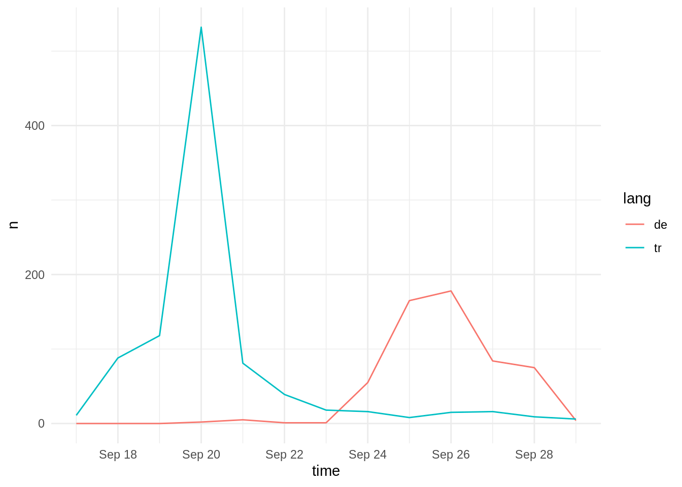
… unfortunately, I didn’t use it last time…
Key Learning: I could have avoided stepping into this trap if I had plotted the distribution of Tweets over time… Exploratory Data Analysis FTW.
This is what I would’ve seen, I had done it right:
joint_collection %>%
  group_by(Discipline) %>%
  rtweet::ts_plot() +
    theme_minimal()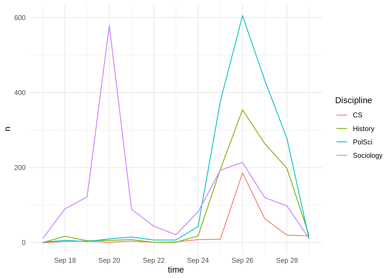
See that left peak around the 20th? Arghhhh!
Time to move on. As we have already set an upper time limit above (filter(created_at < "2018-09-30")), we now only have to include a lower time limit:
joint_collection_week <- joint_collection %>%
  filter(created_at > "2018-09-23")

joint_collection_week %>%
  group_by(lang) %>%
  count() %>%
  filter(n > 2) %>%
  arrange(desc(n)) %>%
knitr::kable(format = "html", digits = 2)| lang | n |
|---|---|
| de | 3068 |
| en | 522 |
| und | 120 |
| tr | 92 |
| nl | 19 |
| sv | 6 |
| es | 4 |
| fr | 4 |
| no | 3 |
Ok, that’s already better, but there are still 92 Turkish Tweets in the sample, and 120 Tweets for lang == "und".
It turns out, however, that
lang == "und"(un)fortunatly meanslanguage undefinedcf. Twitter…
Let’s have a look at the remaining Turkish Tweets and then rebuild our corpora and the document-feature matrix.
joint_collection_week %>%
  filter(lang == "tr") %>%
  select(text) %>%
  head() %>% # for website readability
knitr::kable(format = "html", digits = 2) | text |
|---|
| Çok şükür Allahım… #dgs2018 https://t.co/DAXRFoawzq |
| Mimar sinan güzel sanatlarlı olduk be 😂 #Dgstercih #dgs2018 |
| #dgs2018 derslerden muaf olmak için en çok 5 yıl önce ilgili programdan mezun olmak gerekir şartı var mı arkadaşlar????? Bilen birisi bilgilendirsin lütfen. |
| #dgs2018 AÖF lisans dersleri DGS muafiyetinde kullanıyor mu?? |
| Bilgi Üniversitesi’nde 2000li arkadaşlarımla hazırlık okuyacağım. Yaşlı olmak kontenjanından dışlanmam umarım🙄 #dgs2018 @BiLGiOfficial |
| 4 puan ile iktisat kaybettim sizce ek tercihlerde yazsam çıkar mı?#dgs2018 #DGSekyerleştirme #dgs #DGSE #dgsmovie3 #dgs |
So all the Tweets are exclusivly in Turkish, and it is more than appropriate to exclude them from our analysis here AND in my preceding blog post. (Update incoming!)
But who’s going to tell the German Sociologists that my report from last week had to be corrected and that they didn’t perform that well, actually …!?
Key learning: Never rely on blind/nummeric analysises only. Always do some qualitative exploration and check for plausibility - even when it’s “only” for a blog!!!
4.2 Removing Turkish accounts
First, let’s get list of all the Users who where part of the Turkish #dgs2018 sample (and since I’ve updated the previous post, I have collected some Turkish hashtags for lang=="und", so we’ll just re-use this filter here.)
tr_user <- dgs_collection %>%
  filter(str_detect(text,"yks2018|yksdil|dgsankara|cumhuriyetüniversitesi|DanceKafe") | lang == "tr") %>%
  select(user_id) %>%
  distinct()
tr_user %>% count() %>%
knitr::kable(format = "html", digits = 2)| n |
|---|
| 529 |
Now, we’ll anti_join() the dgs_collection with this list
dgs_collection %>% anti_join(tr_user, by = "user_id") %>% count() %>%
knitr::kable("html")| n |
|---|
| 686 |
Let’s compare with the simpler filter(lang!="tr") approach
dgs_collection %>%
  filter(lang != "tr") %>%
  count() %>%
knitr::kable(format = "html", digits = 2)| n |
|---|
| 717 |
That’s a difference of another ~30 Tweets. Nice. We’ll use that in a minute.
5 Rebuild the Corpus without Tweets with lang=="tr"
There is two ways to do that. One is lazy and one is more replication-friendly. I’ll mention the lazy one, but will continue with the more robust approach
The Lazy Way
(Two lazy ways, actually)
As we know that the Turkish Tweets are exclusively in the Sociology Corpus, we could just rebuild the dgs_corpus and then rebuild the joint_corpus with:
joint_corpus <- dvpw_corpus +
                dgs_corpus +
                hist_corpus +
                inf_corpus +
                mixed_corpus
An even easier way would be to filter out Turkish Tweets from the already existing joint_corpus with quanteda::corpus_subset():
joint_corpus %>% corpus_subset(joint_corpus$documents$lang != "tr")However, if you have been jumping back and forth within this post (or .Rmd Notebook), then you (=me) might have lost track of the various manipulations and state differences (i.e. think of custom_stopwords). Plus, the dgs_corpus would still need attention, too, and as we’ve filtered out a lot of Tweets by setting a lower time limit, the common time period for the corpora would differ, too. BAD!
So let’s rebuild the corpora from scratch.
5.1 Re-Build individual Corpora from Scratch
We’ll just add filter(created_at > "2018-09-23") and for the sake of robustness, we’ll filter all corpora for lang != "tr", and anti_join(dgs_corpus) with tr_user.
As I want both, discipline-specific copora with “multidisciplinary Tweets” and a redundancy-free joint corpus, I’ll build the corpora in two steps.
dvpw_corpus <- dvpw_collection %>%
  filter(created_at > "2018-09-23" & lang != "tr") %>% # combined filter()
  # anti_join(mixed_collection, by = "status_id") %>%
  corpus(docid_field = "status_id", text_field = "text")
  ## not totally sure about the effect of setting text_field = "text"
docvars(dvpw_corpus, "Discipline") <- "PolSci"

dgs_corpus <- dgs_collection %>%
  filter(created_at > "2018-09-23" & lang != "tr") %>%
  # anti_join(mixed_collection, by = "status_id") %>%
  anti_join(tr_user, by = "user_id") %>%
  corpus(docid_field = "status_id", text_field = "text")
docvars(dgs_corpus, "Discipline") <- "Sociology"

hist_corpus <- hist_collection %>%
  filter(created_at > "2018-09-23" & lang != "tr") %>%
  # anti_join(mixed_collection, by = "status_id") %>%
  corpus(docid_field = "status_id", text_field = "text")
docvars(hist_corpus, "Discipline") <- "History"

inf_corpus <- inf_collection %>%
  filter(created_at > "2018-09-23" & lang != "tr") %>%
  # anti_join(mixed_collection, by = "status_id") %>%
  corpus(docid_field = "status_id", text_field = "text")
docvars(inf_corpus, "Discipline") <- "CS"

mixed_corpus <- mixed_collection %>%
  filter(created_at > "2018-09-23" & lang != "tr") %>%
  corpus(docid_field = "status_id", text_field = "text") # 42 docs!
docvars(mixed_corpus, "Discipline") <- "Mixed"
Of course, eventually, we should update and
rm()all the obselete *_collection objects or simply consolidate all the “valid” Tweets in a .rds file. However, I’m not so much into editing raw-ish / original data, so doing that is up to you.
5.2 Create Joint Corpus
joint_corpus <- dvpw_corpus +
                dgs_corpus +
                hist_corpus +
                inf_corpus # 3,748 docs

joint_corpus <- joint_corpus %>% corpus_subset(!(docnames(joint_corpus) %in% mixed_collection$status_id)) # 3,706 docs

joint_corpus <- joint_corpus + mixed_corpus #3,748 docs
6 3rd Attempt @ dfm() Building
joint_dfm <- dfm(joint_corpus,
                # groups = "Discipline",
                 remove = c(stopwords("german"),
                            stopwords("english"),
                            custom_stopwords,
                            min_nchar = 3),
                 remove_punct = TRUE,
                 remove_url = TRUE,
                # remove_numbers = TRUE,
                 tolower = TRUE,
                 verbose = TRUE)
## Creating a dfm from a corpus input...## ... lowercasing## ... found 3,748 documents, 16,371 features## ... removed 608 features
## ... created a 3,748 x 15,763 sparse dfm
## ... complete.
## Elapsed time: 0.58 seconds.We’re down to 15763 features from 3748 documents (Tweets) and were able to get rid of 608 features with the iteratively refined approach.
And as we might want to use a grouped dfm for group comparisons (and dfm_group doesn’t seem to work for me here), we’ll create a custom grouped one, too.
## not working:
# dfm_group(joint_dfm, groups = "Discipline")
# OR
# dfm_group(joint_dfm, groups = c("Discipline"))
# OR
# dfm_group(joint_dfm, groups = docvars(joint_dfm, "Discipline"))
#> Error in qatd_cpp_is_grouped_numeric(as.numeric(x), group) :
#>  (list) object cannot be coerced to type 'double'

joint_dfm_grouped <- dfm(joint_corpus,
                 groups = "Discipline",
                 remove = c(stopwords("german"),
                            stopwords("english"),
                            custom_stopwords,
                            min_nchar = 3),
                 remove_punct = TRUE,
                 remove_url = TRUE,
                # remove_numbers = TRUE,
                 tolower = TRUE,
                 verbose = FALSE) #for website readability
7 Some quick Analyses
7.3 Top Features
Without Hashtags and Twitter @Nicks
# {r results="asis"}
features <- dfm_select(joint_dfm, pattern = list('#*',"@*"),
                       selection = "remove",
                       min_nchar = 3)
topfeatures(features, 40) %>%
knitr::kable("html")| x | |
|---|---|
| panel | 167 |
| demokratie | 142 |
| thema | 93 |
| democracy | 86 |
| sektion | 76 |
| münster | 73 |
| diskussion | 69 |
| kongress | 67 |
| frankfurt | 65 |
| danke | 64 |
| vortrag | 63 |
| spannende | 60 |
| digitale | 59 |
| soziologie | 59 |
| frage | 58 |
| findet | 55 |
| grenzen | 55 |
| gesellschaft | 55 |
| political | 54 |
| spricht | 54 |
| prof | 54 |
| historiker | 54 |
| stand | 53 |
| 2018 | 51 |
| forschung | 51 |
| fragen | 51 |
| freuen | 50 |
| steinmeier | 50 |
| deutschen | 49 |
| politikwissenschaft | 46 |
| geht’s | 45 |
| arbeit | 45 |
| german | 44 |
| new | 44 |
| digitalen | 43 |
| historikertag | 43 |
| rede | 42 |
| geschichte | 42 |
| democratic | 41 |
| eigentlich | 40 |
7.4 Top Features per Discipline
# {r results="asis"}
features <- dfm_select(joint_dfm, pattern = list('#*',"@*"),
                       selection = "remove",
                       min_nchar = 3)
topfeatures(features, 20, groups = "Discipline") %>%
map(knitr::kable, "html")| x | |
|---|---|
| demokratie | 130 |
| panel | 105 |
| democracy | 84 |
| frankfurt | 60 |
| political | 51 |
| grenzen | 49 |
| steinmeier | 47 |
| politikwissenschaft | 45 |
| democratic | 41 |
| kongress | 38 |
| rede | 36 |
| frage | 35 |
| representation | 34 |
| diskussion | 34 |
| thema | 31 |
| politik | 29 |
| podiumsdiskussion | 29 |
| bundespräsident | 28 |
| need | 28 |
| dvpw | 27 |
| x | |
|---|---|
| soziologie | 55 |
| vortrag | 32 |
| kongress | 26 |
| göttingen | 23 |
| panel | 17 |
| spannende | 17 |
| gesellschaft | 15 |
| gruppe | 15 |
| session | 14 |
| raum | 14 |
| plenum | 14 |
| sektion | 13 |
| danke | 12 |
| freuen | 12 |
| forschung | 12 |
| thema | 12 |
| diskussion | 12 |
| sozialen | 12 |
| vogel | 12 |
| woche | 11 |
| x | |
|---|---|
| münster | 67 |
| sektion | 56 |
| historiker | 49 |
| historikertag | 41 |
| digitale | 40 |
| geschichte | 36 |
| panel | 33 |
| geschichtswissenschaft | 30 |
| stand | 29 |
| poster | 29 |
| thema | 28 |
| van | 25 |
| danke | 22 |
| forschung | 21 |
| geht’s | 21 |
| digitalen | 21 |
| history | 21 |
| gespaltene | 21 |
| freuen | 20 |
| findet | 19 |
| x | |
|---|---|
| thema | 21 |
| prof | 16 |
| zukunft | 15 |
| digitale | 14 |
| digitalisierung | 13 |
| informatik | 13 |
| panel | 12 |
| stefan | 12 |
| data | 12 |
| berlin | 11 |
| diskussion | 11 |
| ullrich | 11 |
| science | 10 |
| keynote | 10 |
| digital | 9 |
| amt | 9 |
| ranga | 9 |
| erklärt | 8 |
| arbeit | 8 |
| gesellschaft | 8 |
| x | |
|---|---|
| woche | 3 |
| findet | 3 |
| tweets | 3 |
| minuten | 3 |
| gibts | 3 |
| digitalen | 3 |
| frankfurt | 2 |
| kolleg | 2 |
| sehen | 2 |
| kongresswoche | 2 |
| good | 2 |
| laufen | 2 |
| gemeinsam | 2 |
| interessant | 2 |
| begriff | 2 |
| deutlich | 2 |
| stärker | 2 |
| derzeit | 2 |
| politikwissenschaftler | 2 |
| digitalisierung | 2 |
There are still a couple features which would qualify for being removed (such as “unsere”, “mal”, “schon”), but we will take care of that with the super-useful
quanteda::dfm_trim(<term_freq>)threshold-based feature selection.
Plus, removing or parsing hashtags and applying
dfm(stem = TRUE)would largely increase descriptive accuracy
7.5 Network of feature co-occurrences
topfeats <- names(topfeatures(joint_dfm, 60))
textplot_network(dfm_select(joint_dfm, topfeats), min_freq = 0.8)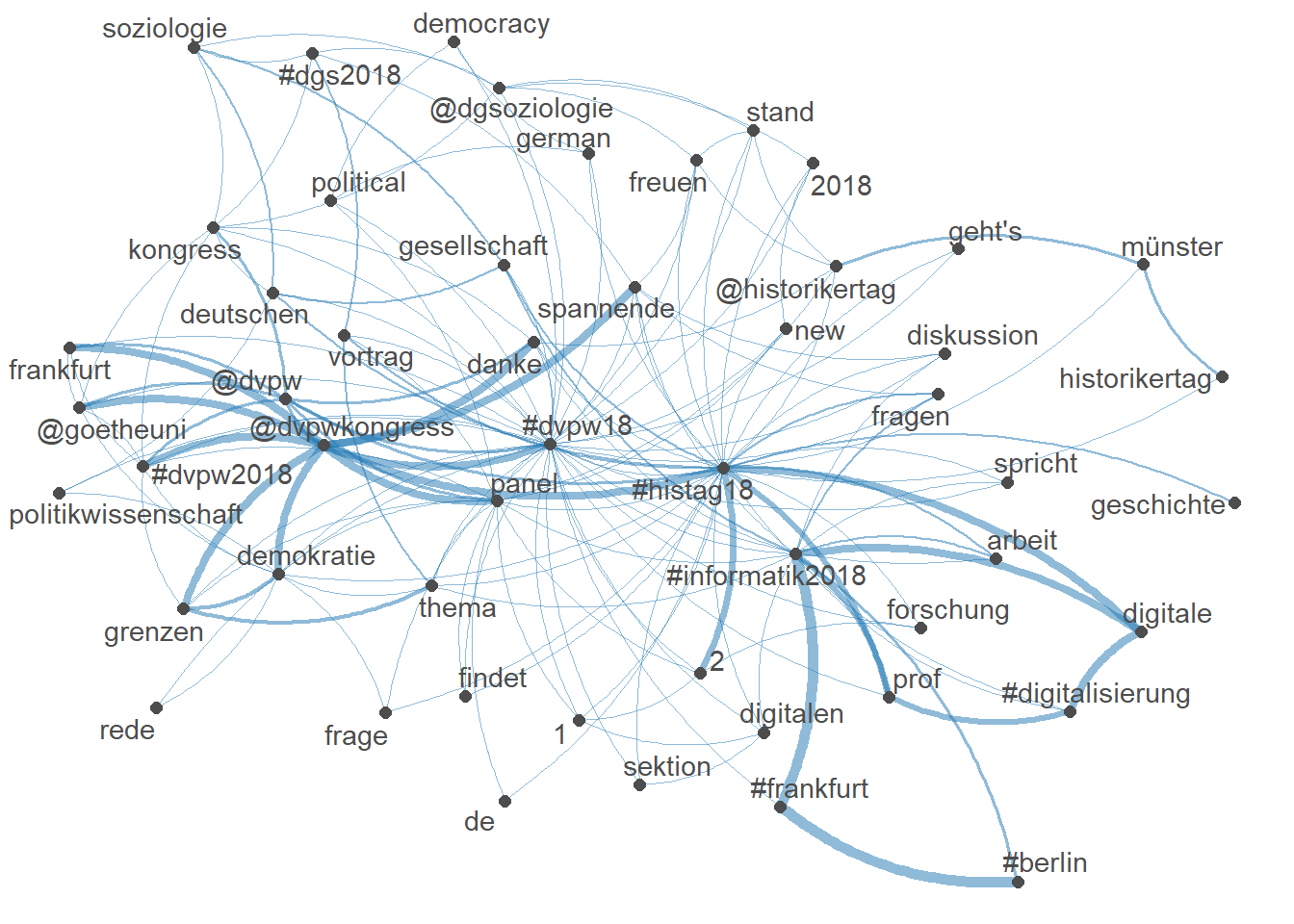
7.6 Grouped wordcloud of features
“wordcloud, where the feature labels are plotted with their sizes proportional to their numerical values in the dfm” (Vignette for
quanteda::textplot_wordcloud)
textplot_wordcloud(joint_dfm_grouped,
                   comparison = TRUE,
                   min_size = 0.5,
                   max_size = 3,
                   max_words = 60)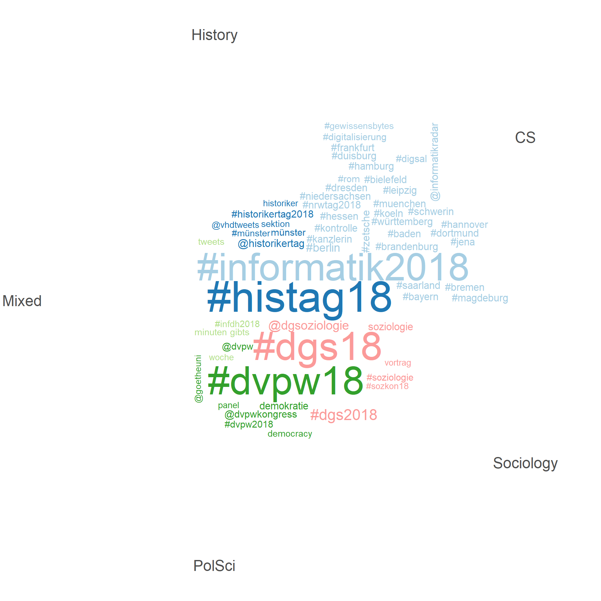
8 What’s next?
Topic Modelling!
Now that I had to spend quite an amount of time on data processing, cleaning, and eventually building a usable dfm, the actual analysis of the contents remains a #TODO
However, I learned a lot doing this today, and I hope that it became obvious that dealing with text as data is not to be underestimated.