[R] Election Hacking: Exploring 10 Million Tweets from the Russian Internet Research Agency Dataset, Pt. 1 - Apporaching 5.3GB in R
Abstract / TL;DR
Post updated with data from the full 5.3GB CSV file from the "Internet Research Agency" dataset

(Creation Date of Top 15 Accounts in the IRA Dataset)
A bit over a week ago, Twitter’s new-ish Elections integrity team released two datasets with “all the accounts and related content associated with potential information operations that we have found on our service since 2016.”
In particular, this is what we are talking about:
“Our initial disclosures cover two previously disclosed campaigns, and include information from 3,841 accounts believed to be connected to the Russian Internet Research Agency [also known as IRA], and 770 accounts believed to originate in Iran.” (Twitter’s Election Integrity Team)
For a bit of a context on the IRA’s activities and the Russian Influence Operation in general, Mashable offers a nice overview.
The IRA zip alone is 1.24 GB big! Let’s dive in and explore. Before we can start with any analysis, automated or not, we have to inspect and prepare the data - remember: EDA FTW!
Anyways, a dataset of this size is a perfect exercise in data wrangling and exploratory analysis with tools from the galactic tidyverse. So what I’m aiming to highlight with this post, is my more or less systematic approach to turning an granular dataset with millions of observations into something more useful (and reliable!) for further in-depth analysis.
1 Data Preperation
You can get the data from here:
- source: https://about.twitter.com/en_us/values/elections-integrity.html#data
- IRA CSV ZIP: https://storage.googleapis.com/twitter-election-integrity/hashed/ira/ira_tweets_csv_hashed.zip
- README: https://storage.googleapis.com/twitter-election-integrity/hashed/Twitter_Elections_Integrity_Datasets_hashed_README.txt
library(tidyverse)First, we need to unpack the .zip file and then read the .csv file into R.
csvfile <- "ira_tweets_csv_hashed.csv"
data_raw <- read_csv("ira_tweets_csv_hashed.csv")

# Just for comparison
data2_raw <- data.table::fread(csvfile,
                          encoding = "UTF-8",
                          # na.strings = ",,",
                          verbose = TRUE)
At first – I (like others) – was getting an CRC error message when unpacking the zip file. The resulting CSV was only 1.17 GB big, so that were not all the Tweets from the IRA dataset. After upgrading
7-ziptov18.05unpacking thezipresults in a 5.3 GB big CSV, which is quite a difference I’d say :)
data.tableis by light years the fastest method, butread_csv()gives meNA’s without an extra hassle whiledata.table::fread()seems to be ignoring any patterns forna.strings. Therefore I’ll be working with the data object fromread_csv()here. Sinceread_csv()is rather slow with aCSVthis big, you can speed up your exploration if you save the data object as an.rdsor.RDatafile.
data_path <- here::here("data", "IRA_Tweets", "/")
# if (!dir.exists(data_path)) dir.create(data_path)
# saveRDS(data_raw, str_c(data_path, "infoops_data.rds"))
data_raw <- readRDS(str_c(data_path, "infoops_data.rds"))
With a dataset this big, skimr::skim() is just perfect (and it’s output much more functional in RStudio)!
data_raw %>% skimr::skim_to_wide() %>% knitr::kable("html")| type | variable | missing | complete | n | min | max | empty | n_unique | median | mean | sd | p0 | p25 | p50 | p75 | p100 | hist |
|---|---|---|---|---|---|---|---|---|---|---|---|---|---|---|---|---|---|
| character | account_language | 0 | 9041308 | 9041308 | 2 | 5 | 0 | 11 | NA | NA | NA | NA | NA | NA | NA | NA | NA |
| character | hashtags | 2378775 | 6662533 | 9041308 | 2 | 156 | 0 | 244865 | NA | NA | NA | NA | NA | NA | NA | NA | NA |
| character | in_reply_to_userid | 8503421 | 537887 | 9041308 | 2 | 64 | 0 | 82809 | NA | NA | NA | NA | NA | NA | NA | NA | NA |
| character | is_retweet | 0 | 9041308 | 9041308 | 4 | 5 | 0 | 2 | NA | NA | NA | NA | NA | NA | NA | NA | NA |
| character | latitude | 9036529 | 4779 | 9041308 | 3 | 19 | 0 | 2752 | NA | NA | NA | NA | NA | NA | NA | NA | NA |
| character | longitude | 9036529 | 4779 | 9041308 | 3 | 18 | 0 | 2807 | NA | NA | NA | NA | NA | NA | NA | NA | NA |
| character | poll_choices | 9040172 | 1136 | 9041308 | 5 | 80 | 0 | 708 | NA | NA | NA | NA | NA | NA | NA | NA | NA |
| character | retweet_userid | 5708124 | 3333184 | 9041308 | 2 | 64 | 0 | 204289 | NA | NA | NA | NA | NA | NA | NA | NA | NA |
| character | tweet_client_name | 40341 | 9000967 | 9041308 | 3 | 32 | 0 | 333 | NA | NA | NA | NA | NA | NA | NA | NA | NA |
| character | tweet_language | 296106 | 8745202 | 9041308 | 2 | 3 | 0 | 58 | NA | NA | NA | NA | NA | NA | NA | NA | NA |
| character | tweet_text | 0 | 9041308 | 9041308 | 1 | 710 | 0 | 6598905 | NA | NA | NA | NA | NA | NA | NA | NA | NA |
| character | urls | 1640484 | 7400824 | 9041308 | 2 | 2057 | 0 | 2760160 | NA | NA | NA | NA | NA | NA | NA | NA | NA |
| character | user_display_name | 0 | 9041308 | 9041308 | 5 | 64 | 0 | 3664 | NA | NA | NA | NA | NA | NA | NA | NA | NA |
| character | user_mentions | 5047231 | 3994077 | 9041308 | 3 | 808 | 0 | 570293 | NA | NA | NA | NA | NA | NA | NA | NA | NA |
| character | user_profile_description | 1371499 | 7669809 | 9041308 | 1 | 160 | 0 | 2597 | NA | NA | NA | NA | NA | NA | NA | NA | NA |
| character | user_profile_url | 7146952 | 1894356 | 9041308 | 22 | 23 | 0 | 200 | NA | NA | NA | NA | NA | NA | NA | NA | NA |
| character | user_reported_location | 1526654 | 7514654 | 9041308 | 2 | 30 | 0 | 608 | NA | NA | NA | NA | NA | NA | NA | NA | NA |
| character | user_screen_name | 0 | 9041308 | 9041308 | 6 | 64 | 0 | 3667 | NA | NA | NA | NA | NA | NA | NA | NA | NA |
| character | userid | 0 | 9041308 | 9041308 | 9 | 64 | 0 | 3667 | NA | NA | NA | NA | NA | NA | NA | NA | NA |
| Date | account_creation_date | 0 | 9041308 | 9041308 | 2009-04-24 | 2018-04-03 | NA | 653 | 2014-03-28 | NA | NA | NA | NA | NA | NA | NA | NA |
| integer | follower_count | 0 | 9041308 | 9041308 | NA | NA | NA | NA | NA | 8670.2 | 22146.39 | 0 | 346 | 842 | 4486 | 257638 | ▇▁▁▁▁▁▁▁ |
| integer | following_count | 0 | 9041308 | 9041308 | NA | NA | NA | NA | NA | 2522.47 | 5028.83 | 0 | 284 | 618 | 2014 | 74664 | ▇▁▁▁▁▁▁▁ |
| integer | like_count | 2673 | 9038635 | 9041308 | NA | NA | NA | NA | NA | 4 | 290.31 | 0 | 0 | 0 | 0 | 325826 | ▇▁▁▁▁▁▁▁ |
| integer | quote_count | 2673 | 9038635 | 9041308 | NA | NA | NA | NA | NA | 0.2 | 13.07 | 0 | 0 | 0 | 0 | 11633 | ▇▁▁▁▁▁▁▁ |
| integer | reply_count | 2673 | 9038635 | 9041308 | NA | NA | NA | NA | NA | 0.28 | 7.41 | 0 | 0 | 0 | 0 | 3249 | ▇▁▁▁▁▁▁▁ |
| integer | retweet_count | 2673 | 9038635 | 9041308 | NA | NA | NA | NA | NA | 3.46 | 140.33 | 0 | 0 | 0 | 0 | 123617 | ▇▁▁▁▁▁▁▁ |
| numeric | in_reply_to_tweetid | 8775100 | 266208 | 9041308 | NA | NA | NA | NA | NA | 6.1e+17 | 1.3e+17 | 0 | 5.7e+17 | 6.3e+17 | 6.6e+17 | 1e+18 | ▁▁▁▁▆▇▁▁ |
| numeric | quoted_tweet_tweetid | 8853395 | 187913 | 9041308 | NA | NA | NA | NA | NA | 8e+17 | 8.7e+16 | 1.8e+09 | 7.7e+17 | 8.1e+17 | 8.5e+17 | 1e+18 | ▁▁▁▁▁▂▇▂ |
| numeric | retweet_tweetid | 5708124 | 3333184 | 9041308 | NA | NA | NA | NA | NA | 6.7e+17 | 1.2e+17 | 100 | 5.7e+17 | 6.5e+17 | 7.9e+17 | 1e+18 | ▁▁▁▁▇▅▆▁ |
| numeric | tweetid | 0 | 9041308 | 9041308 | NA | NA | NA | NA | NA | 6.4e+17 | 1.6e+17 | 1.7e+09 | 5.3e+17 | 6.2e+17 | 7.8e+17 | 1e+18 | ▁▁▁▃▇▅▅▁ |
| POSIXct | tweet_time | 0 | 9041308 | 9041308 | 2009-05-09 | 2018-06-21 | NA | 1788062 | 2015-07-17 | NA | NA | NA | NA | NA | NA | NA | NA |
We can already make some interesting observations from this summary alone:
- The IRA dataset consist of
1.899.5959.041.308 Tweets in5158 languages, from3.4603.667 unique accounts and 11 account languages. That’s pretty “diverse” but also quite complex. $is_retweethas only 2 unique values, so it’s obviously a Boolean ->mutate()- There’s
1.899.5959.041.308 observations for$tweet_text, but only1.634.9426.598.905 are unique. This huge delta just screams: spam bots and/or coordinated campaigns! - only
50K266K Tweets are replies -> rather few interactions - there are some prominent accounts with up to 257K followers
743.8282.760.160 URLs to explore- we can see from
$retweet_useridthat apparently,703.4673.333.184 Tweets are just Retweets and not unique/original Tweets. - if we were to try to classify accounts by profile description, there’s a corpus of
2.4512.597 unique profile descriptions ($user_profile_description) and 200 unique$user_profile_urls - all the
$*_tweetidvars were read as numeric, which we’ll also need to change, as IDs are supposed to be unique identifiers and not continuous values ->mutate() - the Tweets were posted in the period from 2009-05-09 (!) to 2018-06-21, with the median around 2015-07-17
- half of the accounts were created on or after 2014-03-28. Like there was an upcoming election or a referendum or something :)
- there are 608 unique account locations (shared by an unknown number of those 3.667 accounts at this point), and there are 4.779 geolocated Tweets. That’s not much, but we could try to double-check these locations with the respective
$account_languagevalues.
That should give us enough leads for an initial inquiry. Let’s continue with the data preparation and address what we have discovered so far.
1.1 Change Variable Types
convert $is_retweet into a boolean
data_raw$is_retweet <- as.logical(data_raw$is_retweet)convert $*_tweetid vars into strings
data_raw <- data_raw %>%
  mutate_at(vars(ends_with("tweetid")),
            funs(as.character))
Now we can skim just the $*_tweetid vars and $is_retweet
data_raw %>%
  select(is_retweet, ends_with("tweetid")) %>%
  skimr::skim_to_wide(noten_raw) %>%
knitr::kable("html")| type | variable | missing | complete | n | min | max | empty | n_unique | mean | count |
|---|---|---|---|---|---|---|---|---|---|---|
| character | in_reply_to_tweetid | 8775100 | 266208 | 9041308 | 1 | 19 | 0 | 236322 | NA | NA |
| character | quoted_tweet_tweetid | 8853395 | 187913 | 9041308 | 10 | 18 | 0 | 144609 | NA | NA |
| character | retweet_tweetid | 5708124 | 3333184 | 9041308 | 3 | 19 | 0 | 1725841 | NA | NA |
| character | tweetid | 0 | 9041308 | 9041308 | 10 | 19 | 0 | 9035946 | NA | NA |
| logical | is_retweet | 0 | 9041308 | 9041308 | NA | NA | NA | NA | 0.37 | FAL: 5708124, TRU: 3333184, NA: 0 |
Ok, now we know that 3.333.184 (~1/3) Tweets are Retweets (of 1.725.841 unique Tweets). Good to know for any Natural Language Processing Method which depends on statistics, i.e. Topic Modelling, or when building a corpus for descriptive analyses.
1.2 Remove Duplicates
It’s probably more efficient to remove duplicates as the first step. This reduces the data object we’re working with.
data_unique <- data_raw %>% filter(is_retweet == FALSE)Now we’re down to 5707611 unique Tweets in 57 Tweet languages by 3548 Users with 11 account languages.
1.3 Reduce/Recode Language Variables
$tweet_language
data_unique %>%
  group_by(tweet_language) %>%
  count() %>%
  filter(n > 1000) %>%
  arrange(desc(n)) %>%
knitr::kable(format = "html")| tweet_language | n |
|---|---|
| ru | 2839622 |
| en | 2178309 |
| NA | 285539 |
| und | 119098 |
| de | 86259 |
| uk | 49889 |
| bg | 36576 |
| ar | 35811 |
| es | 8402 |
| in | 7543 |
| fr | 7501 |
| sr | 5604 |
| tl | 5176 |
| ht | 4944 |
| et | 4920 |
| sk | 2982 |
| tr | 2903 |
| da | 2699 |
| ro | 2517 |
| it | 2493 |
| nl | 2292 |
| cy | 2214 |
| sl | 2123 |
| pt | 1857 |
| fi | 1414 |
| pl | 1325 |
| sv | 1191 |
| lt | 1190 |
| no | 1135 |
| ja | 1117 |
That’s quite a lot, even if we only consider Tweet languages with n > 1000 Tweets.
merge NA and und[defined]
data_unique <- data_unique %>%
  mutate(tweet_language = if_else(is.na(tweet_language), "und", tweet_language))
recode all langs with n < 5000 as “other”
We need to reduce the scope of Tweet languages for now. 5000 is only slightly less than 1% of the unique Tweets, so this sounds like a good threshold.
# I'm very sure that there's a more elegant solution for mutating observations row-wise based on grouped counts... However, whatever works, works.

other_langs <- data_unique %>%
  group_by(tweet_language) %>%
  count() %>%
  filter(n < 5000) %>%
  select(tweet_language)
data_unique <- data_unique %>%
mutate(tweet_language =
if_else(tweet_language %in% other_langs$tweet_language, "other_44",
tweet_language))n_distinct(data_unique$tweet_language)## [1] 12We’re down to 13 language categories for the Tweets. That’s far better!
$account_language
data_unique %>%
  group_by(account_language) %>%
  distinct(userid) %>%
  count() %>%
  arrange(desc(n)) %>%
knitr::kable("html")| account_language | n |
|---|---|
| en | 2214 |
| ru | 982 |
| es | 194 |
| de | 107 |
| ar | 21 |
| fr | 11 |
| it | 7 |
| en-gb | 6 |
| zh-cn | 3 |
| uk | 2 |
| id | 1 |
So there’s 11 account languages. I’m going to focus on languages with n > 100 accounts, and recode the rest as “other_6” (since we can assume “uk” == “en-gb”, that’s one language less).
other_langs_acc <- data_unique %>%
  distinct(userid, .keep_all = TRUE) %>%
  group_by(account_language) %>%
  count() %>%
  filter(n < 100) %>%
  select(account_language)

data_unique <- data_unique %>%
  mutate(account_language =
           if_else(account_language %in% other_langs_acc$account_language, "other_6",
                                  account_language))
n_distinct(data_unique$account_language)
## [1] 5Great! Now we’re down to 5 account languages.
1.4 IRA Dataset Languages: Summary
Let’s see how many different languages we have by now.
unique(c(data_unique$tweet_language, data_unique$account_language))## [1] "ru" "bg" "en" "und" "other_44" "de"
## [7] "uk" "tl" "es" "ar" "fr" "in"
## [13] "sr" "other_6"Now let’s create a preliminary overview.
data_count_by_tweet_lang <- data_unique %>%
  # filter(is_retweet == TRUE) %>%
  group_by(tweet_language) %>%
  distinct(tweetid) %>%
  count() %>%
  rename(Tweets = n)

data_count_by_account_lang <- data_unique %>%
  # filter(is_retweet == TRUE) %>%
  group_by(account_language) %>%
  distinct(userid) %>%
  count() %>%
  rename(Accounts = n)

lang_stats <- full_join(data_count_by_tweet_lang, data_count_by_account_lang,
  by = c("tweet_language" = "account_language")) %>%
  rename(Language = tweet_language) %>%
  mutate(
    T.Share = round(Tweets / sum(.$Tweets, na.rm = TRUE) * 100, 2),
    A.Share = round(Accounts / sum(.$Accounts, na.rm = TRUE) * 100, 2)
  ) %>%
  select(Language, Tweets, T.Share, Accounts, A.Share) %>%
  arrange(desc(Accounts))
lang_stats %>%
knitr::kable("html",
format.args = list(
big.mark = ".",
decimal.mark = ","),
caption = "#TwitterDump 2018 – Russian InfoOP Dataset: Languages (unique Tweets)"
)| Language | Tweets | T.Share | Accounts | A.Share |
|---|---|---|---|---|
| en | 2.178.206 | 38,16 | 2.214 | 62,40 |
| ru | 2.839.362 | 49,75 | 982 | 27,68 |
| es | 8.402 | 0,15 | 194 | 5,47 |
| de | 86.258 | 1,51 | 107 | 3,02 |
| other_6 | NA | NA | 51 | 1,44 |
| ar | 35.811 | 0,63 | NA | NA |
| bg | 36.575 | 0,64 | NA | NA |
| fr | 7.501 | 0,13 | NA | NA |
| in | 7.543 | 0,13 | NA | NA |
| other_44 | 42.795 | 0,75 | NA | NA |
| sr | 5.604 | 0,10 | NA | NA |
| tl | 5.176 | 0,09 | NA | NA |
| uk | 49.887 | 0,87 | NA | NA |
| und | 404.557 | 7,09 | NA | NA |
That’s already interesting, but let’s not jump to conclusion about who tweeted in what language, yet… This summary alone does enable us to claim that, for instance, Russian accounts where responsible for all the Russian Tweets, and so on.
What’s really striking is that 50% of the Tweets from this 9M Tweets IRA dataset are in Russian (or at least labelled as such), which does not quite fit the dominant narrative of a solely US-centric information operation. These numbers show that Russia’s activities were concered with Russian-speaking people as much as with an English-speaking audience (among German and Spanish).
Check for any remaining language NA’s
data_unique %>% filter(is.na(tweet_language) | is.na(account_language)) %>%
  count()
## # A tibble: 1 x 1
## n
## <int>
## 1 0That’s great news so far!
(Optional: recode if(tweet_lang == NA &/| user_lang == NA))
Since we’ve reduced our dataset and already recoded the NAs, this step is not necessary anymore (before that, I worked without is_retweet == FALSE and things looked a bit different). However, I’m just leaving the syntax here, since it might be useful to others (and to myself).
data_recoded <- data_unique %>%
  mutate(tweet_language = if_else(is.na(tweet_language) & is.na(account_language),
                                  "und",
                            if_else(is.na(tweet_language) & !is.na(account_language),
                                    account_language,
                          tweet_language)
                          )
         ) %>%
  mutate(account_language = if_else(is.na(tweet_language) & is.na(account_language),
                                  "und",
                              if_else(is.na(account_language) & !is.na(tweet_language),
                                      tweet_language,
                            account_language)
                            )
         )
This is a good moment in our data preparation cycle to create a hardcopy of our processed
data_uniqueobject in a.rdsfile. This way, we won’t have to redo all the wrangling and recoding we did so far, and can just start with any in-depth analysis by loading the object withdata_unique <- readRDS(file). ANd we can reduce our local in-memory load byrm(data_raw)
# data_path <- here::here("data", "IRA_Tweets", "/")
# if (!dir.exists(data_path)) dir.create(data_path)
saveRDS(data_unique, str_c(data_path, "infoops_data_processed.rds"))
rm(data_raw)
data_unique <- readRDS(str_c(data_path, "infoops_data_processed.rds"))
2 Who tweeted in what language?
Now it’s about time to look into which account language groups tweeted in what languages.
2.1 Create Language-specific Subsets
This is also a good moment to create language-specific or other intereting subsets from our refined dataset.
German subset
german_subset <- data_unique %>% filter(tweet_language == "de" | account_language == "de")The German subset has 98064 Tweets by 782 users.
Undefined Subset
undefined_subset <- data_unique %>%
  filter(tweet_language == "und" | account_language == "und" |
           is.na(tweet_language) | is.na(account_language))
The undefined (“und” & “NA”) subset has 404557 Tweets by 2867 users.
2.2 Summary Plots: Languages & General Activity
data_unique %>%
  group_by(tweet_language) %>%
  summarise(n = n()) %>%
  mutate(
    share = n / sum(n),
    tweet_language = case_when(
      tweet_language == "" ~ "unspec.",
      tweet_language == "und" ~ "undef.",
      TRUE ~ tweet_language
    )
  ) %>%
  arrange(desc(n)) %>%
  ggplot(aes(area = share)) +
  treemapify::geom_treemap(aes(fill = n), alpha = 0.8) +
  treemapify::geom_treemap_text(
    aes(label = paste0(tweet_language, "\n(", round(share * 100, 1), "%)"))
  ) +
  scale_fill_viridis_c(direction = -1, option = "D") +
  labs(
    title = "#TwitterDump 2018 – Russian InfoOP Dataset: Shares of Languages (Tweets)",
    subtitle = str_c("Total of ",
      n_distinct(data_unique$tweetid), " unique Tweets (no RTs) from ",
      n_distinct(data_unique$userid), " unique Users"
    ),
    caption = str_c("@fubits")
  ) +
  guides(fill = FALSE)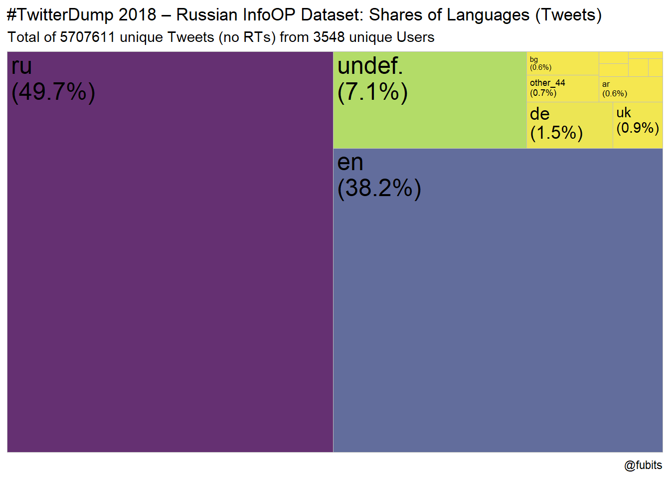
data_unique %>%
  group_by(account_language) %>%
  summarise(n = n()) %>%
  mutate(
    share = n / sum(n),
    account_language = case_when(
      account_language == "" ~ "unspec.",
      account_language == "und" ~ "undef.",
      TRUE ~ account_language
    )
  ) %>%
  arrange(desc(n)) %>%
  ggplot(aes(area = share)) +
  treemapify::geom_treemap(aes(fill = n), alpha = 0.8) +
  treemapify::geom_treemap_text(
    aes(label = paste0(account_language, "\n(", round(share * 100, 1), "%)"))
  ) +
  scale_fill_viridis_c(direction = -1, option = "D") +
  labs(
    title = "#TwitterDump 2018 – Russian InfoOP Dataset: Shares of Languages (Accounts)",
    subtitle = str_c("Total of ",
      n_distinct(data_unique$tweetid), " unique Tweets (no RTs) from ",
      n_distinct(data_unique$userid), " unique Users"
    ),
    caption = str_c("@fubits")
  ) +
  guides(fill = FALSE)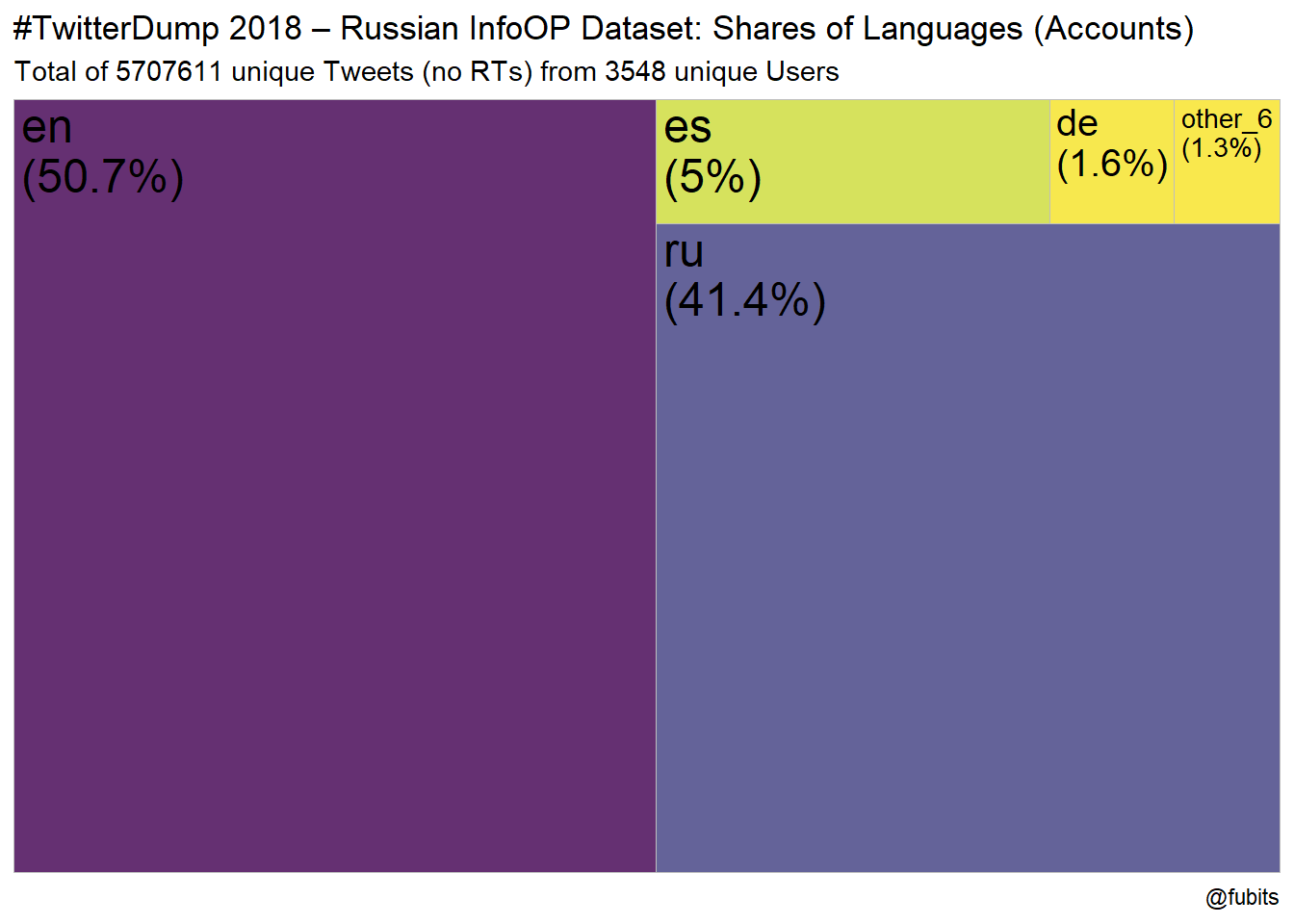
2.2.1 Consolidating Tweet Languages per Account
data_counts <- data_unique %>%
  group_by(userid) %>%
  mutate(Account_Lang = account_language) %>%
  summarise(
    Created = unique(account_creation_date),
    Account_Lang = unique(Account_Lang),
    Tweets = n(),
    RT = sum(retweet_count),
    Follower = unique(follower_count),
    Following = unique(following_count),
    Influence = (((Follower + 1) / (Following + 1)) + (Follower + 1)),
    Tweet_Langs = list(tweet_language),
    Tweet_Langs_Counts = list(unlist(Tweet_Langs) %>% fct_count())
  ) %>%
  arrange(desc(Tweets))
Now the $Tweet_Langs var contains a list of all Tweet Languages from every single Tweet posted by an Account. Compare the number of $Tweets with the length of the vector (in the list) further below.
For $Tweet_Langs_Counts, we have utilized the quite elegant forcats::fct_count() which gives us a list of the aggregated language counts.
So the first User in our dataset - who has tweeted a total of 95210 times - has been busy in 6 languages. Impressive language skills :)
data_counts[1,]$Tweet_Langs_Counts[[1]] %>% knitr::kable("html")| f | n |
|---|---|
| bg | 536 |
| en | 2 |
| ru | 93478 |
| sr | 26 |
| uk | 1093 |
| und | 75 |
And this is what this tibble looks like (without $userid and $Tweet_Langs for better Website readability):
data_counts %>%
  select(-userid, -Tweet_Langs) %>%
head(10) %>% knitr::kable("html", digits = 0)| Created | Account_Lang | Tweets | RT | Follower | Following | Influence | Tweet_Langs_Counts |
|---|---|---|---|---|---|---|---|
| 16237 | ru | 95210 | 188332 | 15753 | 6862 | 15756 | list(f = 1:6, n = c(536, 2, 93478, 26, 1093, 75)) |
| 14553 | ru | 68784 | 11700 | 1543 | 34 | 1588 | list(f = 1:13, n = c(3, 488, 14, 290, 12, 10, 1, 153, 26633, 90, 9, 686, 40395)) |
| 16625 | en | 64495 | 1898 | 791 | 2 | 1056 | list(f = 1:11, n = c(17, 1105, 44410, 766, 753, 2561, 13267, 1, 1474, 6, 135)) |
| 16309 | en | 59397 | 44258 | 66980 | 10500 | 66987 | list(f = 1:8, n = c(64, 58607, 94, 113, 44, 339, 42, 94)) |
| 16204 | en | 53781 | 29179 | 23595 | 13665 | 23598 | list(f = 1:8, n = c(75, 53067, 90, 135, 28, 308, 9, 69)) |
| 16227 | en | 52838 | 19670 | 29357 | 6720 | 29362 | list(f = 1:8, n = c(129, 51643, 148, 147, 68, 463, 92, 148)) |
| 17093 | ru | 50224 | 1526 | 423 | 187 | 426 | list(f = 1:7, n = c(247, 1, 2, 49436, 8, 442, 88)) |
| 16431 | en | 46738 | 3619 | 13358 | 13851 | 13360 | list(f = 1:8, n = c(46, 45943, 149, 115, 48, 293, 43, 101)) |
| 16195 | en | 46572 | 25119 | 35988 | 11010 | 35992 | list(f = 1:8, n = c(72, 45890, 56, 163, 58, 264, 34, 35)) |
| 16626 | ru | 46440 | 24685 | 13913 | 1650 | 13922 | list(f = 1:7, n = c(344, 1, 4, 45398, 19, 560, 114)) |
I’ll get back to this in a minute. Let’s now visualize the general characteristics of all accounts in the IRA dataset.
2.2.2 General Activity Plots
ggplot(data_counts, aes(x = Follower, y = Following)) +
  geom_point(aes(size = Tweets, color = userid, alpha = Influence)) +
  scale_color_viridis_d(direction = -1) +
  scale_alpha_continuous(range = c(0.3,1),
                         breaks = scales::pretty_breaks(5)) +
  scale_size(range = c(1,5), labels = scales::number_format(big.mark = ".",
                                                    decimal.mark = ",")) +
  scale_x_continuous(breaks = scales::pretty_breaks(6),
                     labels = scales::number_format(big.mark = ".",
                                                    decimal.mark = ",")) +
  scale_y_continuous(breaks = scales::pretty_breaks(6),
                     labels = scales::number_format(big.mark = ".",
                                                    decimal.mark = ",")) +
  coord_fixed() +
  theme_minimal() +
  labs(
    title = "#TwitterDump 2018 – Russian InfoOP Dataset: Account Stats",
    subtitle = str_c("Total of ",
      n_distinct(data_unique$tweetid), " unique Tweets (no RTs) from ",
      n_distinct(data_unique$userid), " unique Users"
    ),
    caption = str_c("@fubits"),
    #x = "",
    # y = "",
    size = "# of Tweets",
    alpha = "Alpha: # Retweets"
  ) +
    guides(color = FALSE, alpha = FALSE)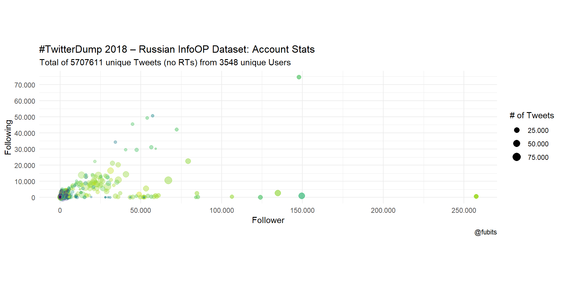
From what we can see here, we have quite an amount of “influencers” - accounts with lots of followers and low rates of following others.
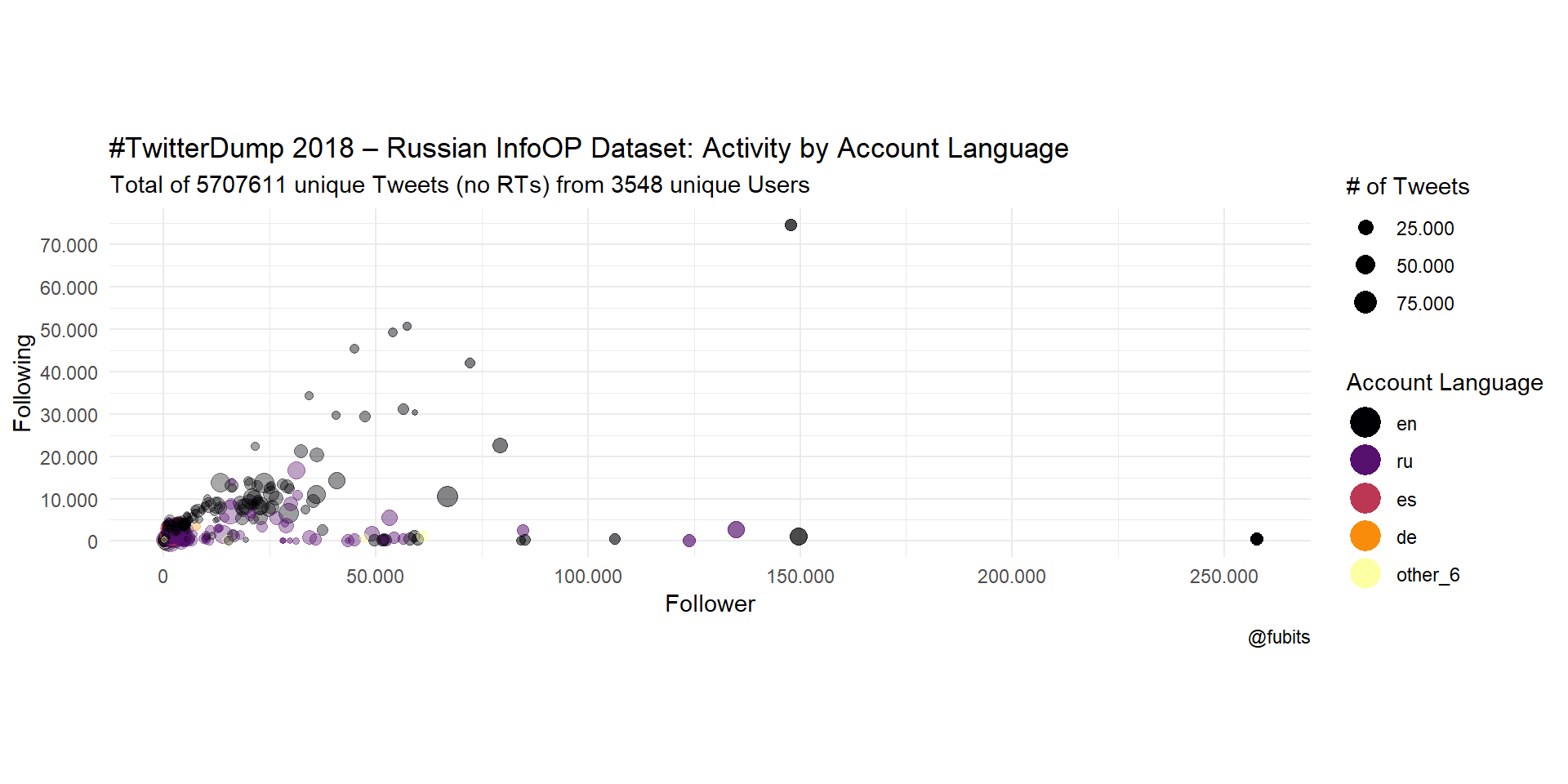
What if we look at the account languages?
ggplot(data_counts, aes(x = Follower, y = Following)) +
  geom_point(aes(size = Tweets, color = fct_infreq(Account_Lang), alpha = Influence)) +
  scale_color_viridis_d(option = "B", direction = 1) +
  scale_alpha_continuous(range = c(0.3,1),
                         labels = scales::number_format(big.mark = ".",
                                                    decimal.mark = ",")) +
  scale_size(range = c(1,5), labels = scales::number_format(big.mark = ".",
                                                    decimal.mark = ",")) +
  scale_x_continuous(breaks = scales::pretty_breaks(6),
                     labels = scales::number_format(big.mark = ".",
                                                    decimal.mark = ",")) +
  scale_y_continuous(breaks = scales::pretty_breaks(6),
                     labels = scales::number_format(big.mark = ".",
                                                    decimal.mark = ",")) +
  coord_fixed() +
  theme_minimal() +
  labs(
    title = "#TwitterDump 2018 – Russian InfoOP Dataset: Activity by Account Language",
    subtitle = str_c("Total of ",
      n_distinct(data_unique$tweetid), " unique Tweets (no RTs) from ",
      n_distinct(data_unique$userid), " unique Users"
    ),
    caption = str_c("@fubits"),
    #x = "",
    # y = "",
    size = "# of Tweets",
    color = "Account Language"
  ) +
    guides(alpha = FALSE,
           colour = guide_legend(override.aes = list(size = 5, stroke = 1.5))
           )
And now let’s just look at when the most influential accounts were created.
influencers <- data_counts %>%
  arrange(desc(Influence)) %>%
  top_n(15, Influence)

data_counts %>%
  arrange(desc(Influence)) %>%
  ggplot(data = ., aes(x = Follower, y = Following)) +
    geom_point(aes(size = Tweets, color = fct_infreq(Account_Lang), alpha = Influence)) +
    ggrepel::geom_label_repel(data = influencers,
                            aes(label = lubridate::year(Created),
                                fill = Account_Lang),
                            alpha = 0.7) +
    scale_color_viridis_d(option = "B", direction = 1) +
    scale_alpha_continuous(range = c(0.3,1),
                           labels = scales::number_format(big.mark = ".",
                                                      decimal.mark = ",")) +
    scale_size(range = c(1,5), labels = scales::number_format(big.mark = ".",
                                                      decimal.mark = ",")) +
    scale_x_continuous(breaks = scales::pretty_breaks(6),
                       labels = scales::number_format(big.mark = ".",
                                                      decimal.mark = ",")) +
    scale_y_continuous(breaks = scales::pretty_breaks(6),
                       labels = scales::number_format(big.mark = ".",
                                                      decimal.mark = ",")) +
    coord_fixed() +
    theme_minimal() +
    labs(
      title = "#TwitterDump 2018 – Russian InfoOP Dataset: Top 15 (Influence) - Account Creation Date",
      subtitle = str_c("Total of ",
        n_distinct(data_unique$tweetid), " unique Tweets (no RTs) from ",
        n_distinct(data_unique$userid), " unique Users"
      ),
      caption = str_c("@fubits"),
      #x = "",
      # y = "",
      size = "# of Tweets",
      color = "Account Language"
    ) +
      guides(alpha = FALSE,
             colour = FALSE)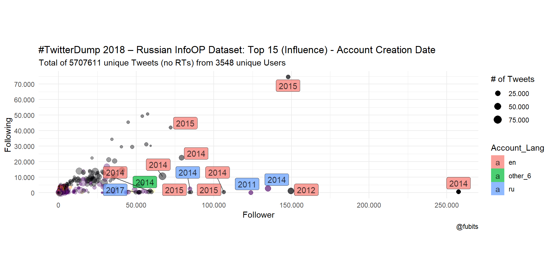
Interesting, one of the most influential accounts is neither Russian nor English-speaking!
data_counts %>%
  arrange(desc(Influence)) %>%
  select(userid, Account_Lang, Follower, Following) %>%
head(15) %>% knitr::kable("html")| userid | Account_Lang | Follower | Following |
|---|---|---|---|
| 2527472164 | en | 257638 | 544 |
| 508761973 | en | 149672 | 1024 |
| 4224729994 | en | 147767 | 74664 |
| 449689677 | ru | 123989 | 10 |
| 2808833544 | ru | 134805 | 2796 |
| 2648734430 | en | 106462 | 386 |
| 890237781737435138 | ru | 51964 | 0 |
| 3676820373 | en | 85293 | 316 |
| 3729867851 | en | 84167 | 143 |
| 2665564544 | ru | 84642 | 2575 |
| 2882331822 | en | 79152 | 22607 |
| 4272870988 | en | 72121 | 42080 |
| 2752677905 | en | 66980 | 10500 |
| 2518710111 | other_6 | 60869 | 1246 |
| 2573726278 | en | 59724 | 556 |
2518710111 is not hashed :) Let’s find out who this is!
data_raw %>% filter(userid == 2518710111) %>% select(userid, user_display_name, user_screen_name, account_language) %>% head(1) %>% knitr::kable("html")| userid | user_display_name | user_screen_name | account_language |
|---|---|---|---|
| 2518710111 | Вестник Новосибирска | NovostiNsk | en-gb |
“Вестник Новосибирска” - Newspaper of Novosibirsk - doesn’t sound too British :) the account has been suspended by Twitter, btw.
What about accounts with the most Tweets?
data_counts %>%
  ggplot(data = ., aes(x = Follower, y = Following)) +
    geom_point(aes(size = Tweets, color = fct_infreq(Account_Lang), alpha = RT)) +
    ggrepel::geom_label_repel(data = data_counts[1:15,],
                            aes(label = lubridate::year(Created),
                                fill = Account_Lang),
                            alpha = 0.7) +
    scale_color_viridis_d(option = "B", direction = 1) +
    scale_alpha_continuous(range = c(0.3,1),
                           labels = scales::number_format(big.mark = ".",
                                                      decimal.mark = ",")) +
    scale_size(range = c(1,5), labels = scales::number_format(big.mark = ".",
                                                      decimal.mark = ",")) +
    scale_x_continuous(breaks = scales::pretty_breaks(6),
                       labels = scales::number_format(big.mark = ".",
                                                      decimal.mark = ",")) +
    scale_y_continuous(breaks = scales::pretty_breaks(6),
                       labels = scales::number_format(big.mark = ".",
                                                      decimal.mark = ",")) +
    coord_fixed() +
    theme_minimal() +
    labs(
      title = "#TwitterDump 2018 – Russian InfoOP Dataset: Top 15 (# Tweets) - Account Creation Date",
      subtitle = str_c("Total of ",
        n_distinct(data_unique$tweetid), " unique Tweets (no RTs) from ",
        n_distinct(data_unique$userid), " unique Users"
      ),
      caption = str_c("@fubits"),
      #x = "",
      # y = "",
      size = "# of Tweets",
      color = "Account Language"
    ) +
      guides(alpha = FALSE,
             colour = FALSE)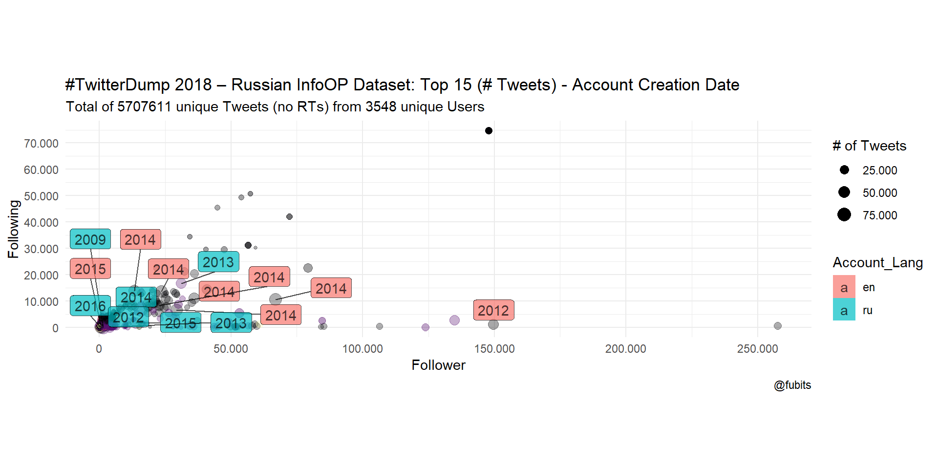
We can see from both plots that the most influential or active accounts were created in 2014 or later, and that the relation between Russian- and English-labelled accounts is rather balanced in terms of max. Tweet numbers. However, English-speaking accounts are more dominant in terms of numeric dominance (Following/Followers).
2.3 Languages: Accounts vs Tweets
Now it’s time to have look at the account language to tweet languages relations.
This is what the Top 20 (of 57) language combinations look like:
data_unique %>%
  group_by(account_language, tweet_language) %>%
  count() %>%
  arrange(desc(n)) %>%
  head(20) %>%
knitr::kable("html", caption = "Top 20 Language Combinations from the IRA Dataset")| account_language | tweet_language | n |
|---|---|---|
| ru | ru | 1985869 |
| en | en | 1842222 |
| en | ru | 836074 |
| ru | und | 310192 |
| es | en | 275732 |
| en | und | 80810 |
| de | de | 78301 |
| other_6 | en | 51105 |
| en | other_44 | 35542 |
| en | ar | 33013 |
| ru | uk | 28038 |
| ru | bg | 21923 |
| en | uk | 21520 |
| other_6 | ru | 17679 |
| en | bg | 14539 |
| de | und | 10387 |
| ru | en | 8500 |
| en | es | 7259 |
| en | de | 6637 |
| en | in | 6407 |
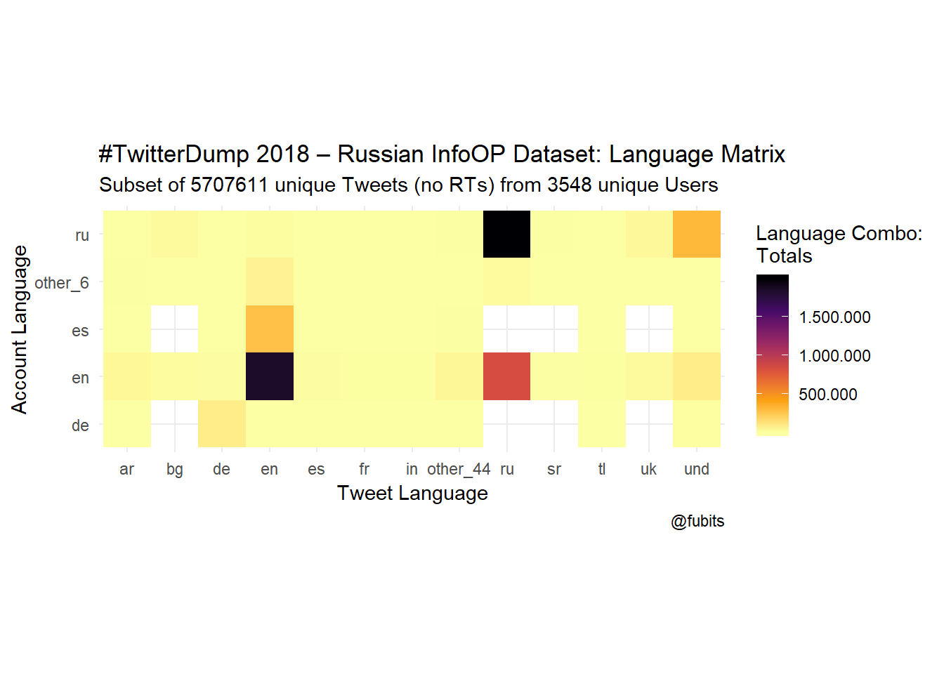
Ok, so we probably could have expected that Russian and English speaking accounts would mostly tweet in their respective languages. But who would have suspected that 185.803 Russian language tweets were posted by English-speaking accounts? Right :)
Now let’s visualize all the 57 Account Language -> Tweet Language combinations. For an easier understanding of these plots, just keep in mind that Tweets are posted by accounts, so the Tweet language (bottom) is our dependent variable here.
data_unique %>%
  group_by(account_language, tweet_language) %>%
  count() %>%
  arrange(desc(n)) %>%
    ggplot() +
    geom_tile(aes(x = tweet_language,
                  y = account_language,
                  fill = n)) +
    scale_fill_viridis_c(option = "B", direction = -1,
                         breaks = scales::pretty_breaks(4),
                         labels = scales::number_format(big.mark = ".",
                                                        decimal.mark = ",")) +
    coord_fixed() +
    theme_minimal() +
    labs(
      title = "#TwitterDump 2018 – Russian InfoOP Dataset: Language Matrix",
      subtitle = str_c(
        "Subset of ", n_distinct(data_unique$tweetid),
        " unique Tweets (no RTs) from ",
        n_distinct(data_unique$userid), " unique Users"
      ),
      caption = str_c("@fubits"),
      fill = "Language Combo:\nTotals",
      x = "Tweet Language",
      y = "Account Language"
    )
data_unique %>%
  group_by(account_language, tweet_language) %>%
  count() %>%
  arrange(desc(n)) %>%
    ggplot() +
    geom_tile(aes(x = tweet_language,
                  y = account_language,
                  fill = n/sum(n))) +
    scale_fill_viridis_c(option = "B", direction = -1,
                         breaks = scales::pretty_breaks(6),
                         labels = scales::percent_format(accuracy = 1)) +
    coord_fixed() +
    theme_minimal() +
  # theme(axis.text.x = element_text(angle = 45, vjust = 1, hjust = 1)) +
    labs(
      title = "#TwitterDump 2018 – Russian InfoOP Dataset: Language Matrix",
      subtitle = str_c(
        "Subset of ", n_distinct(data_unique$tweetid),
        " unique Tweets (no RTs) from ",
        n_distinct(data_unique$userid), " unique Users"
      ),
      caption = str_c("@fubits"),
      fill = "Language Combo:\nShare of Total"
    )
Alright, that’s enough exploration and heavy data wrangling for today. Stay tuned for Part 2: Content Analysis
Here’s just a teaser of what is expecting us:
data_unique %>%
  filter(tweet_language == "ru") %>%
  select(tweet_text) %>%
  head(10) %>%
knitr::kable("html")| tweet_text |
|---|
| Серебром отколоколило http://t.co/Jaa4v4IFpM |
| Предлагаю судить их за поддержку нацизма, т.к. они отказались его осуждать!! #STOPNazi |
| Двойная утопия, или Нет у Европы Трампа, кроме Путина https://t.co/MbxCpuLdDl |
| Генпрокуратура назвала взносы на капремонт неконституционными https://t.co/IOiSR4kssB |
| Кировский пасхальный обед один из самых дешевых в стране https://t.co/11se2vaZJS |
| В Кирове на два месяца будет ограничено движение по улице Кольцова https://t.co/iRT0jWIS9z |
| Пятница в Кирове: солнечный чай и любимое занятие https://t.co/jATZrjoAdy |
| ИнстаКиров: топ прокачанных парней в спортзале http://t.co/q45lGEaHla |
| Что обсуждают в Кирове: убийство женщины и концерт “Арии” https://t.co/MUhZaTSXAA |
| В музее Циолковского открылась выставка, посвященная нашему земляку Юрию Тухаринову https://t.co/T3BR53yu7B https://t.co/WDDkBworPE |
Or what about “undefined”
data_unique %>%
  filter(tweet_language == "und") %>%
  select(tweet_text) %>%
  head(10) %>%
knitr::kable("html")| tweet_text |
|---|
| #волгоград #сталинград https://t.co/RCoCV12FP0 |
| *** http://t.co/qpmvojRvYx |
| @stratosathens Strat, Every time we are in the state of burning chemical plants! Why is it happened with us?! |
| http://t.co/RFTj00YJXU |
| https://t.co/pDSEWw50AH |
| http://t.co/yYLD9IhvYO |
| @b059c98801ff33056eb46bee9088256f2b6b85dc8d6926579bf42dbf1b2d9c1a Curiosity «завис» на Марсе из-за сбоя в компьютере |
| @bee7d3ea2fb7ece347e636f3c21b9340e1e17626bfd7543d1d36b51d00d0a4ce Чехия испытывает дефицит российской нефти |
| Автомобиль Дворковича попал в ДТП |
| @050f6f287ff564463cb290ec9933a045e07d0eea41352e3ed893cd570e97adbb “Доктор Питер”: Петербургские инвесторы могут построить в Белоруссии фармацевтический завод #СПб #spb |
Btw, have you already discovered the US-Republican-sponsored (sic!) RussiaTweets.com Project?