[R] Election Hacking: Exploring 10 Million Tweets from the Russian Internet Research Agency Dataset, Pt. 2 - Corpus & DFM
Abstract / TL;DR
This is the sceond part of my "Internet Research Agency" series. We'll encounter in-memory computing problems, address them with tweaks on Windows and Linux, and finally succeed at building a 5.7M x 1.5M big sparse Document-Feature Matrix.

(Weekly per-language activity of specific keywords)
Now that we are done with pre-processing the Internet Research Agency dataset, we can unleash the full R powers and dive into automated content analysis. For a primer, see the following excellent intros and posts re: core NLP concepts, R packages, and tools:
- Emmanuel Ameisen: How to solve 90% of NLP problems: a step-by-step guide (this is a very beginner-friendly overview of key NLP concepts. Not R related, but a great TL;DR primer.)
- Julia Silge: The game is afoot! Topic modeling of Sherlock Holmes stories
- Julia Silge and David Robinson: Text Mining with R - A Tidy Approach
- Cornelius Puschmann: Automatisierte Inhaltsanalyse mit R (in German)
- Kenneth Benoit et al.: quanteda: An R package for the quantitative analysis of textual data
- Benoit et al.? Quanteda vignette: Getting Started with Quanteda
- Nicolas Merz: Using the Manifesto Corpus with quanteda
- Bonus: Carsten Schwemmer (who introduced me to the
Tidyverseand automated content analysis with R, btw!) has build anShinyapp, which enables you to explore Structural Topic Models with a browser-based GUI: stminsights - A Shiny Application for Structural Topic Models
Just a word of caution: Topic Modelling is a statistical method, and doing it the way I’m doing here - on the full 5.7M Tweets corpus OR even on a subset of 2M Tweets without any frequency-based feature reduction (i.e. with
quanteda::dfm_trim()) - will take some time. A lot of time actually. I have a decent Gamer’s Laptop with 16GB RAM, a quad-core Intel i7-7500 CPU and a SSD (SATA tho) - and computing the Topic Model based on the English subset (2M Tweets, with auto-induced K=73 topics, based on 15K features -> cf. upcoming 3rd part of this series) took a whole day (22,5 hours). Don’t try this at home, or without some free AWS credits :)
1 Packages & Data
Let’s get started. Here are some tweaks/tricks/adjustments I discovered while writing this post (i.e., in this 8 years old Stack Overflow thread) in order to increase the computing performance ;)
i.e.:
memory.limit(size = NA)sets the maximum memory limit to what’s ever possible on your system (it’s a bit more complicated on Windows)
You can enforce R’s garabage collection at any time with
gc()(see the vignette for the params); this is esp. helpful afterrm(huge_object)
Save any large output as an
.rdsor.RData(if you can afford) to your hard-drive, clear your environment and start the next step with as low of a RAM footprint as possible.
My key-learning of this post, however: If you’re on Windows, set-up a Linux distro to dual-boot. R is so much more performant on Ubuntu et al. (also with regards to Unicode, path length, memory management and much more) You’ll start the environment with at least 1GB more of free RAM; you’ll have full CLI control over the swap drive/file; and then some more.
Let’s start. Here are the packages we’ll need:
library(tidyverse)
library(quanteda)
quanteda_options("threads" = 4) # 4 is the limit on my Laptop
print(str_c("Threads for Quanteda: ", quanteda_options("threads")))
## [1] "Threads for Quanteda: 4"library(stm)
library(lubridate)Since we’ve already pre-processed the Internet Research Agency dataset, we can just load the exported data object and go on with corpus-building.
data_path <- here::here("data", "IRA_Tweets", "/")
data_unique <- readRDS(str_c(data_path, "infoops_data_processed.rds"))
# devtools::install_github("brooke-watson/BRRR")
BRRR::skrrrahh("flava") # play sound when ready
2 International Corpus: An Exersise in “Too Big for In-Memory”
2.1 Data Exploration: Time-Series Plots
As I didn’t do this in my last post, let’s have a quick look at the time-wise distribution of Tweets in total, and grouped by Tweet and Account languages. This way, we might see what time periods and what languages might be worth special attention.
First, we’ll reduce the observations to language groups and further aggregate on a weekly basis.
IRA_TS <- data_unique %>%
  mutate(tweet_time = as_date(tweet_time),
         week = lubridate::floor_date(tweet_time, "week")) %>%
  group_by(week, account_language, tweet_language) %>%
  count() %>%
  arrange(desc(n))
IRA_TS %>%
head() %>%
knitr::kable("html")| week | account_language | tweet_language | n |
|---|---|---|---|
| 2014-07-13 | ru | ru | 89198 |
| 2015-03-15 | en | en | 71421 |
| 2017-08-13 | es | en | 71037 |
| 2017-08-06 | es | en | 55256 |
| 2014-06-22 | ru | ru | 49209 |
| 2014-08-10 | ru | ru | 46044 |
Now we’ll plot time series grouped by account languages.
IRA_TS %>%
    ggplot() +
      geom_line(aes(x = week, y = n, color = fct_infreq(account_language)),
                alpha = 0.5) +
      scale_color_brewer(palette = "Paired", direction = -1) +
      scale_x_date(limits = c(as_date("2009-01-01"), NA),
                   breaks = scales::date_breaks(width = "1 year"),
                   labels = scales::date_format(format = "%Y"),
                   minor_breaks = "6 months") +
      scale_y_continuous(breaks = scales::pretty_breaks(9),
                         labels = scales::number_format(big.mark = ".",
                                                    decimal.mark = ",")) +
      theme_minimal() +
      labs(
        title = "Russian Internet Agency Dataset: Weekly Activity per Account Language",
        subtitle = str_c(
          "Subset of ", n_distinct(data_unique$tweetid),
          " unique Tweets (no RTs) from ",
          n_distinct(data_unique$userid), " unique Users"
        ),
        caption = "@fubits",
        color = "Account Language",
        x = "",         y = "Tweets"        ) +
      guides(colour = guide_legend(override.aes = list(size = 5, stroke = 1.5)))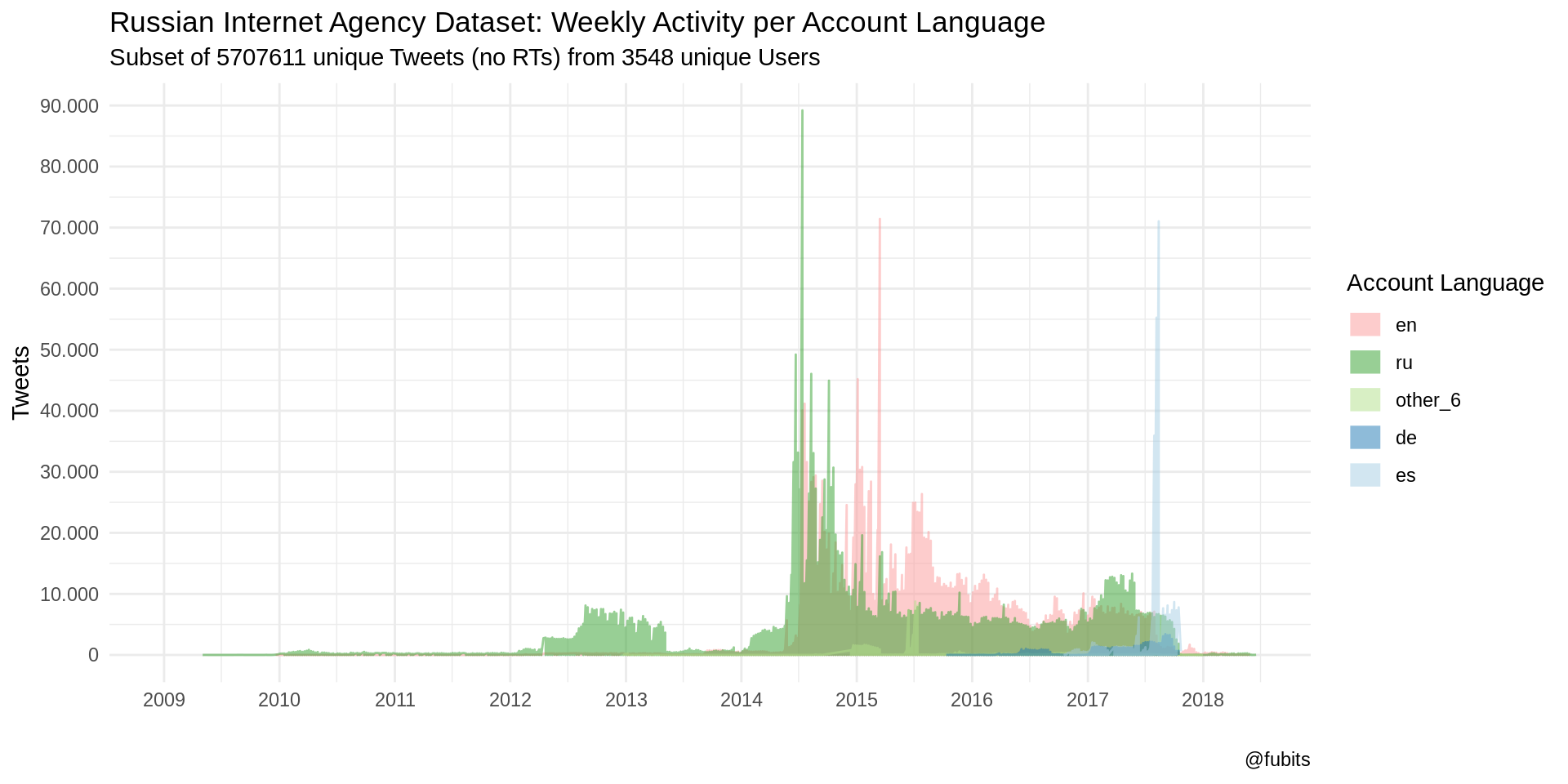
Well that’s some interesting peaks - first “ru”, then “en”, than a little phase with “ru” followed by “es” (as in Español)! We can neglect everything before 2012 for now, so the following plots should become a bit more detailed.
Let’s see what we can observe by plotting the Tweet Languages and inspect the top peaks’ dates. To further reduce noise, we’ll filter out languages with less than 500 Tweets per week from 2012 on (as we have aggregated the Tweets on a weekly basis, in fact, only week-wise values will be filtered out).
IRA_TS %>%
  filter(week > "2011-12-25" & n > 500) %>%
    ggplot() +
      geom_line(aes(x = week, y = n, color = fct_infreq(tweet_language)),
                alpha = 0.5) +
      scale_color_brewer(palette = "Paired", direction = -1) +
      scale_x_date(limits = c(as_date("2011-11-01"), NA),
                   breaks = scales::date_breaks(width = "1 year"),
                   labels = scales::date_format(format = "%Y"),
                   minor_breaks = "6 months") +
      scale_y_continuous(breaks = scales::pretty_breaks(9),
                         labels = scales::number_format(big.mark = ".",
                                                    decimal.mark = ",")) +
      theme_minimal() +
      labs(
        title = "Russian Internet Agency Dataset: Weekly Activity per Tweet Language",
        subtitle = str_c(
          "Subset of ", n_distinct(data_unique$tweetid),
          " unique Tweets (no RTs) from ",
          n_distinct(data_unique$userid), " unique Users"
        ),
        caption = "@fubits",
        color = "Tweet Language",
        x = "",
        y = "Tweets"
        ) +
      guides(colour = guide_legend(override.aes = list(size = 5, stroke = 1.5)))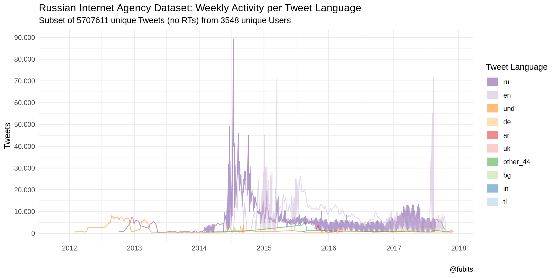
Those patterns are really telling! And we can add one more helper: Text labels (the Mondays for the respective weeks) for those top peaks (global maxima), colored by the respective Account languages. Plus, the real activity starts to gain momentum in 2014, so we should neglect everything beforehand for now
IRA_TS %>%
  filter(week > "2013-12-23" & n > 500) %>%
    ggplot() +
      geom_line(aes(x = week, y = n, color = fct_infreq(tweet_language)),
                alpha = 0.5) +
      geom_point(data = IRA_TS[1:10,], aes(x = week, y = n,
                                          color = fct_infreq(tweet_language)), size = 2) +
      scale_color_brewer(palette = "Paired", direction = -1, aesthetics = c("color", "fill")) +
      ggrepel::geom_label_repel(data = IRA_TS[1:10,],
                                aes(x = week, y = n,
                                    label = str_c(month(week, label = T, abbr = T), "-", day(week)),
                                    fill = account_language),
                                    size = 3) +
      scale_x_date(limits = c(as_date("2013-10-01"), NA),
                   breaks = scales::date_breaks(width = "1 year"),
                   labels = scales::date_format(format = "%Y"),
                   minor_breaks = "6 months") +
      scale_y_continuous(breaks = scales::pretty_breaks(9),
                         labels = scales::number_format(big.mark = ".",
                                                    decimal.mark = ",")) +
      theme_minimal() +
      labs(
        title = "Russian Internet Agency Dataset: Weekly Activity per Language (Top 10 Peaks)",
        subtitle = str_c(
            "Subset of ", n_distinct(data_unique$tweetid),
            " unique Tweets (no RTs) from ",
            n_distinct(data_unique$userid), " unique Users", "; Label: week's Monday; Label fill: Account language"
          ),
        caption = "@fubits",
        color = "Language",
        x = "",
        y = "Tweets"
        ) +
      guides(color = guide_legend(override.aes = list(size = 5, stroke = 0)),
             fill = FALSE)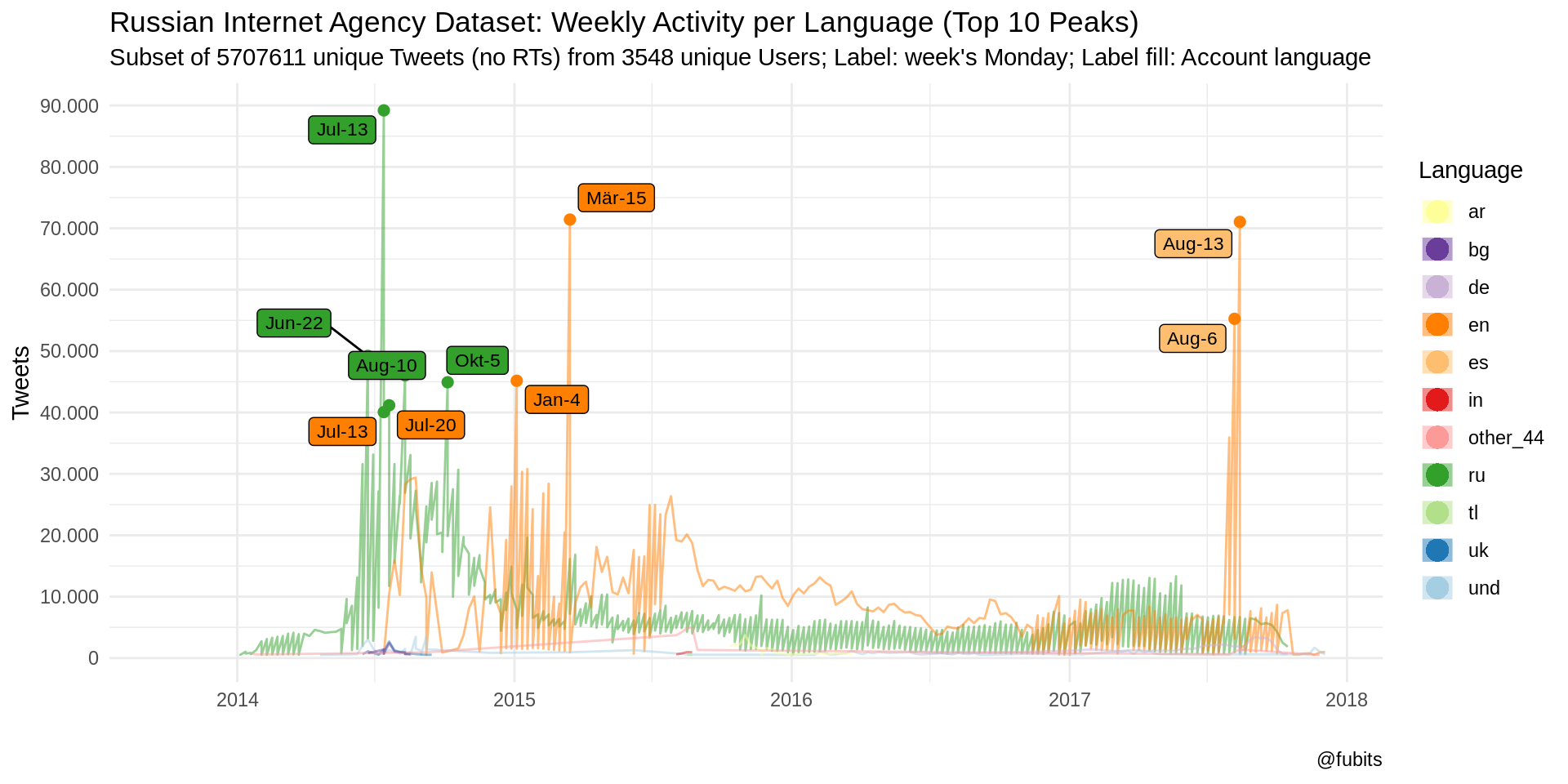
Technically, we could re-do this for all peaks of any particular Tweet or Account language and find out more about the particular events (i.e. German-language Tweets peaking around the Federal Elections in autum 2017 - barely visibly with this color palette) with the help of Wikipedia’s super-handsome current events portal.
For instance, we can observe Russian-language Tweets starting to peak at the beginning of 2014:
- post-Maidan, the Ukraine-Russia conflict just entered a full-fledged armed conflict period, complemented by Russia’s Annexation of Crimea et al.
- on 17 July Malaysia Airlines Flight MH17 was shot down over Ukraine (cf. Bellingcat’s OSINT work).
As for the English-language Tweets (attributed to the Russian “Internet Research Agency” by Twitter’s Election Intergrity Team in this dataset), we see them gain momentum starting in mid 2014, shortly after the shot-down of MH17…
Beyond that, in 2015:
- the Greeks elected a new Parliament on 4 January
- the Charlie Hebdo attack took place on 7 January,
- the Ferguson unrest had another bloody month in March
- well… and on 16 June 2015, Trump announced his presidential campaign.
Post election, English-language Tweets calmed down and didn’t re-peak before August 2017:
- on 3 August 2017, “Special counsel Robert Mueller has impaneled a grand jury in Washington, D.C. to investigate allegations of Russia’s interference in the 2016 elections”1
- (and Neymar was bought by PSG for €222 million on the same day, which might explain why Spanish Accounts where most active here)
- on 12 August 2017, “fights break out between white supremacists and counterprotesters in Charlottesville, Virginia, over the removal of the Robert Edward Lee Sculpture.”2.
- on 13 August 2017 the Barcelona attacks happened
As we can see, the activities really peak around certain events, either concerning US-American left-right clashes and other intra-state affairs, or they concern topics with Russian involvement. What’s striking, however, is that the days around the infamous Brexit referendum (23/24 June 2016) are among those time periods with the overall lowest activies.
Just for comparison (of plain numbers to the usefulness of exploration by data visualization), here’s some tables of the data we just visualized. You can easily identify the dates of the events from the numbers alone. But in order to recognize patterns, esp. language patterns, a visual representation is really helpful. However, without this table I probably would have missed the Spanish-language Accounts peaking with Tweets in English in two subsequent weeks…
IRA_TS %>%
  group_by(week, account_language, tweet_language) %>%
  summarise(n = sum(n)) %>%
  arrange(desc(n)) %>%
  head(20) %>%
knitr::kable("html")| week | account_language | tweet_language | n |
|---|---|---|---|
| 2014-07-13 | ru | ru | 89198 |
| 2015-03-15 | en | en | 71421 |
| 2017-08-13 | es | en | 71037 |
| 2017-08-06 | es | en | 55256 |
| 2014-06-22 | ru | ru | 49209 |
| 2014-08-10 | ru | ru | 46044 |
| 2015-01-04 | en | en | 45167 |
| 2014-10-05 | ru | ru | 44925 |
| 2014-07-20 | en | ru | 41167 |
| 2014-07-13 | en | ru | 40059 |
| 2017-07-30 | es | en | 35927 |
| 2014-06-29 | ru | ru | 33153 |
| 2014-08-17 | ru | ru | 33068 |
| 2014-07-27 | en | ru | 31603 |
| 2014-06-15 | ru | ru | 31592 |
| 2015-01-18 | en | en | 30791 |
| 2014-10-19 | ru | ru | 30689 |
| 2015-01-11 | en | en | 30341 |
| 2014-08-24 | en | en | 29403 |
| 2014-08-17 | en | en | 29123 |
Alright. Point made. Let’s continue with preparing our automated content analysis.
rm(IRA_TS) # free up some RAM first2.2 Building a Corpus with Quanteda
We’re going to build a corpus from our dataset, turn the corpus into a sparse Document-Feature Matrix (DFM), reduce unnecessary features (words/tokens) from the DFM and then use the DFM for Structural Topic Modelling.
Now let’s try to do something really naive: We’ll build a corpus from all Tweets - with all languages. This will take a minute ot two (actually: each step took me hours…) with
corpus(), anddfm(), but this way we can explore a lot of presumed topics in various languages early on, and test where the limits of in-memory computing with text as data might be with R (“Big Data calling”)…
Corpus from all Tweets
system.time({ # just measuring run-time
IRA_corpus <- data_unique %>%
  corpus(text_field = "tweet_text",
         docid_field = "tweetid",
         docvars = data_unique, # probably obsolete when docid_field is set
         compress = FALSE # compression is better for in-memory, but will slow down processing
         )
})
BRRR::skrrrahh("flava")
2.2.1 Memory Management
That’s my fairly refined approach (from this post) to work in-memory with as low of a RAM footprint as possible:
- save the data object to the hard-drive with
saveRDS(obj) - clear your R environment with
rm()andgc()( gc := garbage collection) - restart R with
.rs.restartR()orrstudioapi::restartSession()(not sure yet, where they really differ) - load the data object from the hard-drive with
obj <- readRDS() - go on with the next task
save IRA_corpus to HDD
saveRDS(IRA_corpus, str_c(data_path, "IRA_corpus_naive.rds"))
# saveRDS(IRA_corpus, str_c(data_path, "IRA_corpus_naive_compressed.rds"))
clear environment and restart R
rm(data_unique)
rm(IRA_corpus)
gc(full = TRUE, verbose = TRUE)
# .rs.restartR()
rstudioapi::restartSession()
Linux: down to 1.4 GiB
load IRA_corpus from HDD
data_path <- here::here("data", "IRA_Tweets", "/")
IRA_corpus <- readRDS(str_c(data_path, "IRA_corpus_naive.rds"))
# IRA_corpus <- readRDS(stringr::str_c(data_path, "IRA_corpus_naive_compressed.rds"))
BRRR::skrrrahh("flava")
2.3 Corpus Exploration: Keyword-in Context
Now we can explore some specific keywords and their full-text conetxt, i.e. those where we can already assume that they should take up a prominent spot in the corpus.
In particular, I’m interested in the following terms:
- компромат | kompromat (just for you, @RidT)
- soros
- fake news: phrase(“fake news”)
- pee tape: phrase(“pee tape”)
- msm
- hillary | clinton
- nazi
- antifa
- zion
- civil war
- deep state
test kwic() functionality
IRA_corpus %>%
  corpus_subset(tweet_language == "ru" | tweet_language == "en") %>%
  corpus_sample(1000000) %>% # always test with smaller sample
  kwic(c("компромат","kompromat"), window = 10, case_insensitive = TRUE)  %>%
  # vs. kwic(x, phrase("term1 term2"))
  as_tibble() %>% # needed for kwic()
  select(pre:post) %>%
  head(10) %>%
knitr::kable("html")| pre | keyword | post |
|---|---|---|
| Trump wants this fountain to be in charge of Russia’s | Kompromat | on him . https : / / t.co / H8P7CMMxzA |
We’ll put the keywords into a (kwic()-friendly) vector and then do a single run with all keywords instead of repeating this n-times. This will take time and might not work properly without enough RAM.
kwic_keywords <- c(
  c("компромат","kompromat"),
  "soros",
  phrase("fake news"),
  phrase("pee tape"),
  "msm",
  c("hillary", "clinton"),
  "nazi",
  "antifa",
  "zion",
  phrase("civil war"),
  phrase("deep state")
  )
enforce Garbage Collection to free up RAM
gc(full = TRUE, verbose = TRUE)now search for Keywords-in-context from kwic_keywords vector
library(magrittr)
system.time({
  kwic_results <- IRA_corpus %>%
    # corpus_sample(1000000) %>% # Test smale-scale sample first
    quanteda::kwic(kwic_keywords, window = 10, case_insensitive = TRUE)
})

saveRDS(kwic_results, str_c(data_path, "kwic_corpus_naive.rds"))
# this genius thing plays Flavor Flav when the chunk is done
BRRR::skrrrahh("flava")
I was getting this error repeatedly on Windows:Error: cannot allocate vector of size 64.0 Mb Timing stopped at: 1599 562.6 2294
This was the moment where I arrived at my individual “too big for in-memory” point of failure - even with 16GB RAM. After trying out some
memory.size()tricks on Windows, among other things, I decided to change my OS (for R at least) to Ubuntu (MATE 18.10) and set up dual-boot. My first motiviation was to reduce some memory load (i.e. Skype, iTunes, Office et al. all helpers running in the background). Eventually, I had to extend the “in-memory” capacity by creating a dedicated 64GB swap drive on a USB 3.0 thumb drive. As soons as I get hold of a new, bigger, and faster SSD, I’ll have a look at the performance of a SSD-based swap drive.
Visualization
kwic_results <- readRDS(str_c(data_path, "kwic_corpus_naive.rds"))kwic_results %>%
mutate(keyword = tolower(keyword)) %>%
group_by(keyword) %>%
count() %>%
arrange(desc(n)) %>%
knitr::kable("html")| keyword | n |
|---|---|
| clinton | 18216 |
| hillary | 17353 |
| antifa | 6771 |
| fake news | 2897 |
| soros | 2673 |
| msm | 1567 |
| nazi | 1273 |
| deep state | 852 |
| civil war | 741 |
| компромат | 118 |
| zion | 67 |
| pee tape | 7 |
| kompromat | 1 |
This is not as many results as I would have expected. However, this might have been caused by me by not explicitly defining the search pattern as “glob” or “regex”. I’ll re-do this post with better equipment soon-ish.
kwic_results %>%
  filter(keyword == "soros") %>%
  select(pre, keyword, post) %>%
  head(10) %>%
knitr::kable("html")| pre | keyword | post |
|---|---|---|
| Ah_peaceseeker3 AmericanVoterUS KevinDaGunny FoxNews realDonaldTrump Right ? It’s coming from | soros | European ba … https : / / t.co / vdqVmwNR7v |
| MittRomney I’ve learned they’re both antifa’s . I’m positive . | soros | put out ads 7 d … https : / / |
| RT apostlelaurinda : howjohns123 CGHallenbeck RealJamesWoods all funded by | soros | and saudi prince $ $ $ . . . birds |
| TaylorLorenz Another | soros | troll ? Or truly compassionate . These days none of |
| them on the list too . They’re the colluders with | soros | . |
| Soros / Killary gonna take place of ANTIFA ANOTHER 501C | soros | / K … https : / / t.co / U7QhxwnPyN |
| You guys are pushing the antifa agenda . You know | soros | paid off Gov , Mayor & amp ; Police Chief |
| glad you agree . We’re now watching phase 2 of | soros | plan . Destroy US infrastructur … https : / / |
| RT MikeObrigewitch : TeamTrumpAZ No I think obama and | soros | should be removed |
| the entire movement . These kids are being controlled by | soros | via the M … https : / / t.co / |
Now it’s really easy to visualize the distribution of our selected keywords over time and by language and weekly frequency:
kwic_results %>%
  left_join(data_unique, by = c("docname" = "tweetid")) %>%
  select(keyword, tweet_time, account_language, tweet_language) %>%
  mutate(keyword = tolower(keyword), date = floor_date(tweet_time, "week")) %>%
  group_by(keyword, date, account_language) %>%
  count() %>%
  ggplot() +
    geom_point(aes(x = date, y = fct_rev(keyword),
                   color = account_language,
                   size = n), alpha = 0.5) +
    scale_color_brewer(palette = "Paired", direction = 1) +
    labs(title = "Russian Internet Agency Dataset: Selected Keywords - Weekly Activity per Account Language",
         subtitle = str_c("Based on n = ", nrow(kwic_results), " hits from the full IRA dataset"),
         caption = "@fubits",
         x = "Weekly Activity",
         y = "",
         color = "Account\nLanguage") +
    theme_minimal() +
    guides(color = guide_legend(override.aes = list(size = 5,
                                                    stroke = 0,
                                                    alpha = 1)))
The Spanish-language dominance in 2017 looks really weird.
kwic_results %>%
    left_join(data_unique, by = c("docname" = "tweetid")) %>%
    filter(account_language == "es") %>%
    select(account_language, tweet_language, pre, keyword, post, tweet_time) %>%
  head(20) %>%
knitr::kable("html")| account_language | tweet_language | pre | keyword | post | tweet_time |
|---|---|---|---|---|---|
| es | en | SHOCKING : Look What Crooked Favor James Comey Did For | Hillary | Clinton https : / / t.co / weUNOc0m98 | 2017-09-01 16:55:00 |
| es | en | : Look What Crooked Favor James Comey Did For Hillary | Clinton | https : / / t.co / weUNOc0m98 | 2017-09-01 16:55:00 |
| es | en | RT Cernovich : | ANTIFA | , a left wing group , would punch solo #UnitetheRight | 2017-08-12 19:24:00 |
| es | en | #ade BOMBSHELL STUDY : Voter Fraud May Have Resulted in | Hillary | Winning New Hampshire https : / / t.co / a2KZEMQz1B | 2017-07-31 22:31:00 |
| es | en | #darccy Trump Supporters REACT to Mitt Romney PRAISING | ANTIFA | ! https : / / t.co / QGyEnhJWfx #darcy https | 2017-08-17 00:47:00 |
| es | en | #mar RT comermd : | Antifa | Democrats have successfully aligned with Nazi beliefs . Tomecide is | 2017-08-16 17:52:00 |
| es | en | #mar RT comermd : Antifa Democrats have successfully aligned with | Nazi | beliefs . Tomecide is common before destroying a civilization ! | 2017-08-16 17:52:00 |
| es | en | #emel BREAKING : Masked | Antifa | Thugs Pick a FIGHT With Chicago Police https : / | 2017-08-16 15:49:00 |
| es | en | RT stranahan : | Soros | funded spokesman runs from Beth Chapman https : / / | 2017-08-01 03:01:00 |
| es | en | #IStandWithHannity #IStandWithEricBolling Free speech & amp ; truth ! NEVER | Soros | facists seanhannity eri … https : / / t.co / | 2017-08-08 14:29:00 |
| es | en | : What the Dem #Fake Media Is Hiding About the | Clinton | Email Probe https : / / t.co / JviO83XBFA #just | 2017-08-10 11:11:00 |
| es | en | Sorry | Hillary | , Former President Carter Didn’t Vote For You https : | 2017-05-09 12:46:00 |
| es | en | VIDEO : BUTSTED ! Bill | Clinton | Caught Ogling Ivanka Trump While Hillary Looks on in Disgust | 2017-01-21 01:53:00 |
| es | en | : BUTSTED ! Bill Clinton Caught Ogling Ivanka Trump While | Hillary | Looks on in Disgust https : / / t.co / | 2017-01-21 01:53:00 |
| es | en | Trump to Release Unheard | Hillary | Tape … Stunning , Unprecedented https : / / t.co | 2017-05-15 18:40:00 |
| es | en | BREAKING : Man Planning to KILL Trump was | Hillary | Clinton’s Close Friend ! His Plan is SICK … https | 2017-01-22 17:34:00 |
| es | en | Peter Schweizer : | Clinton | Foundation Probe Must Continue - You Can’t Say ’ She | 2016-11-13 01:58:00 |
| es | en | Look What | Antifa | THUGS Did to This Black Student in Charlottesville https : | 2017-08-17 16:48:00 |
| es | en | #adsnn Violent | Antifa | THUG Arrested for Assault in Charlottesville https : / / | 2017-08-14 01:11:00 |
| es | en | There is no one in the | MSM | who will tell the truth - period . Enlist in | 2017-08-18 01:17:00 |
Hm, does not look too Spanish to me. That’s another topic for further exploration and investigation.
#TODO
2.4 Building a 5.7M x 1.5M Sparse Document-Feature Matrix
From a tactical perspective with regards to large corpora and in-memory processing, this particular Stack Overflow introduced an interesting but actually misleading approach for creating a huge dfm: 000andy8484 - Create dfm step by step with quanteda.
After failing to build a dfm from the untouched corpus repeatedly (on Windows & Linux), this SO-post explained how to reduce the number of features in the corpus by tokenizing the texts and removing unwanted tokens before creating the dfm. This way I really gained some momentum for dfm() (by reducing dimensions), but we would also loose the analytic methods / functionality of a corpus object (i.e. kwic()) as we destroy the basic corpus structure (full Tweets in our case) by replacing the texts with tokens. This experiment was more of a performance evaluation than a recommended practice (for now, at least). I ended up with something like a 60M x 1.5M DFM, which obviously shows that I had lost the document-based corpus structure.
Having said that, here’s our regular strategy:
- create untouched corpus (we did this above, already)
remove obsolete tokens from corpus by directly tokenizing the textsremove stopwords from corpus- create dfm from
reduceduntouched corpus - reduce dfm by removing unwanted features (stopwords, URLs, 2-char tokens and so on)
- build dfm subsets for specific analyses
- build topic models with stm() based on variations of the
dfm
Naive Corpus
# data_path <- here::here("data", "IRA_Tweets", "/")
IRA_corpus <- readRDS(stringr::str_c(data_path, "IRA_corpus_naive.rds"))
2.4.1 Stopwords
First of all, we will need to create list of very frequent tokens/words which we can simply filter out from our corpus. This is my current best-practice with regards to stopwords. I’m using three different sources to compile a super-list of stopwords for the languages concerned. (As for “amp”, this is an artifact I encountered in my previous posts: It’s just a left-over of &, which is the HTML entity for string-parsing &, and is created when we use remove_punct = TRUE. Same is true for " and probably some other unparsed/escaped entities in the IRA dataset).
# repo: https://github.com/stopwords-iso
en_stopwords <- readr::read_lines("https://raw.githubusercontent.com/stopwords-iso/stopwords-en/master/stopwords-en.txt")
ru_stopwords <- readr::read_lines("https://raw.githubusercontent.com/stopwords-iso/stopwords-ru/master/stopwords-ru.txt")
de_stopwords <- readr::read_lines("https://raw.githubusercontent.com/stopwords-iso/stopwords-de/master/stopwords-de.txt")

custom_stopwords_en <- unique(c(en_stopwords,
                             tidytext::stop_words$word,
                             quanteda::stopwords("english"))) # only keep uniques
custom_stopwords_ru <- unique(c(ru_stopwords,
                             quanteda::stopwords("russian"))) # only keep uniques
custom_stopwords_de <- unique(c(de_stopwords,
                             quanteda::stopwords("german"))) # only keep uniques

stopwords_extra <- c("amp", "http", "https", "quot")
custom_stopwords_en <- c(custom_stopwords_en, stopwords_extra)
custom_stopwords_ru <- c(custom_stopwords_ru, stopwords_extra)
custom_stopwords_ru <- c(custom_stopwords_ru, stopwords_extra)

rm(en_stopwords) # free up RAM. We'll need it soon-ish
rm(ru_stopwords)
rm(de_stopwords)
2.4.2 Deprecated Approach
Caution: This is the taboo-approach, which I tried out and would not recommend re-doing. It performs. But the analytical value/utility of the output is rather limited!
This task alone would first approach taking up more than 20GB “RAM”" on my Windows OS Laptop and eventually crash, so be warned again: proceed with caution!
On Ubuntu Linux we’ll get along with 9GB-11GB RAM for the same task (corpus building, tokenizing and reducing) without even touching the swap file. The difference is insane… However, this still would not work out for creating a
dfmfrom the untouched, all-tweets corpus. If you want to replicate this, I suggest at least 16GB RAM + 20GB swap memory or 32GB RAM and a regular-sized swap file/drive. SSD performance might be better. Or cloud, if you’re willing (and able) to pay 2-3€/hour for the larger instances…
library(quanteda)
quanteda::quanteda_options("threads" = 4)
system.time({
texts(IRA_corpus) <- quanteda::tokens(IRA_corpus,
                                      remove_twitter = TRUE,
                                      remove_url = TRUE,
                                      remove_punct = TRUE,
                                      remove_numbers = TRUE,
                                      # ngrams = 1:2
                                      )
})
BRRR::skrrrahh("flava")


system.time({
texts(IRA_corpus) <- tokens_remove(texts(IRA_corpus),
                                   c(custom_stopwords_en,custom_stopwords_ru))
})
BRRR::skrrrahh("flava")

saveRDS(IRA_corpus, str_c(data_path, "IRA_corpus_naive_clean.rds"))
BRRR::skrrrahh("flava")

# **Reset session**

rm(data_unique)
rm(IRA_corpus)
rm(custom_stopwords_en)
rm(custom_stopwords_ru)
gc(full = TRUE, verbose = TRUE)
# .rs.restartR()
rstudioapi::restartSession()

data_path <- here::here("data", "IRA_Tweets", "/")
IRA_corpus <- readRDS(str_c(data_path, "IRA_corpus_naive_clean.rds"))
BRRR::skrrrahh("flava")
2.4.3 Regular Approach
Corpus
We already have a plain, untouched corpus object from further above, so we can skip this step.
IRA_corpus <- data_unique %>%
  corpus(text_field = "tweet_text",
         docid_field = "tweetid",
         docvars = data_unique, # probably obsolete when docid_field is set
         compress = FALSE # compression is better for in-memory, but'll slow down processing
         )
Instead, we’ll load the clean, untouched corpus from our HDD and proceed with dfm()
data_path <- here::here("data", "IRA_Tweets", "/")
IRA_corpus <- readRDS(str_c(data_path, "IRA_corpus_naive.rds"))
BRRR::skrrrahh("flava")
Sparse Document-Feature Matrix with quanteda::dfm()
Now we’ll turn the international corpus into a sparse Document-Feature Matrix / Document-Term-Matrix with quanteda::dfm() and include n-grams of 1 and 2 words (bigrams).
My apporach for smaller tasks still is to clear the environment after every big step with
rm()on the objects and enforcinggc(), then.rs.restartR(), and thenreadRDS()the last processed object…
On Windows, this task would slow down first, and then crash, no matter what. Eventually, I was able to get this done by:
- installing Linux/Ubuntu MATE 18.10
- setting up a USB 3.0 thumb drive as a 64GB swap drive (my current SSD is too small for Windows and Ubuntu + swap partition)
- calling
gcinfo(TRUE)to make the garbage collection (gc()) verbose, so that I was able to monitor the memory states - and finally, starting with a clean session (see the steps described just above)
dfm() pt.1
gcinfo(TRUE) # sets gc() to verbose = TRUE; even when output == "FALSE""
system.time({
IRA_dfm <- dfm(
  # corpus_sample(IRA_corpus, 1000000), #always test with small n first
  IRA_corpus, # full corpus
  tolower = TRUE,
  verbose = TRUE,
  min_nchar = 3,
  remove = c(custom_stopwords_en, custom_stopwords_ru, custom_stopwords_de),
  remove_twitter = FALSE,
  remove_numbers = TRUE,
  remove_punct = TRUE,
  remove_url = TRUE)
})
BRRR::skrrrahh("flava")
> Argument min_nchar not used
We’ll keep that in mind…
... created a 5,708,124 x 1,534,498 sparse dfm
Success! Thanks Linux! But don’t forget to save this dfm object!!!
dfm() pt.2
Now we’ll make sure that there are no left-over 1- and 2-character tokens (which are called features from now on) and then save the dfm to our HDD.
rm(IRA_corpus)
IRA_dfm <- dfm_select(IRA_dfm, min_nchar = 3) # double-checking
saveRDS(IRA_dfm, str_c(data_path, "IRA_dfm_naive_clean.rds"))
BRRR::skrrrahh("flava")
gcinfo(FALSE) # turn off verbosing for garbage collection
IRA_dfm <- readRDS(str_c(data_path, "IRA_dfm_naive_clean.rds"))Applying min_nchar = 3 twice actually really helped. Now we are down to a:
5708124 x 1530058 sparse DFM (4.5K features less now).
summary(IRA_dfm)## Length Class Mode
## 8733760791192 dfm S4Holy sh*t. That’s the power of
R+Quanteda+LinuxI guess. So my “little” proof-of-concept experiment worked out. You can build a large dfm from a large corpus without resorting to cloud computing / AWS et al.
Now we can explore a bit more and then proceed over to building a topic model.
2.5 International Tweets: Top-Features
Let’s have a quick look at the most frequent features from all ~5.7M Tweets (in all Tweet languages)
topfeatures(IRA_dfm, 40) %>%
knitr::kable("html")| x | |
|---|---|
| #news | 236677 |
| россии | 115430 |
| сша | 111463 |
| #sports | 96852 |
| trump | 93964 |
| украина | 87824 |
| #politics | 74959 |
| украины | 67625 |
| police | 58584 |
| новости | 57005 |
| украине | 56198 |
| #спб | 52898 |
| #local | 52026 |
| people | 49801 |
| путин | 47521 |
| мнение | 45908 |
| workout | 43647 |
| love | 41963 |
| obama | 39125 |
| #новости | 38359 |
| области | 37143 |
| life | 35277 |
| time | 34470 |
| из-за | 33244 |
| video | 32206 |
| day | 30315 |
| #world | 29351 |
| фото | 27870 |
| президент | 27017 |
| breaking | 26119 |
| #business | 25763 |
| woman | 25379 |
| president | 25149 |
| москве | 24527 |
| порошенко | 24517 |
| u.s | 23593 |
| сирии | 23327 |
| black | 22892 |
| shooting | 22701 |
| house | 22352 |
Funny! Russian terms dominate the international corpus aka Twitter’s “Internet Research Agency” dataset :)What’s also noteworthy, is the top-ranked news hashtag, probably pointing at the proliferation of the “fake news” term.
Now let’s create a subset of our dfm without #hashtags and @account handles for a purer content analysis. It’s a bit redundant, but due to the (in-memory) size of the full-languages dfm (2.8GB with hashtags/accounts; 2.7GB w/o) this is necessary if we want to work with and without Twitter artifacts.
IRA_dfm_no_twitter <- dfm_select(IRA_dfm, pattern = list('#*',"@*"),
                       selection = "remove")
saveRDS(IRA_dfm_no_twitter, str_c(data_path, "IRA_dfm_naive_clean_no_twitter.rds"))
We’ve further reduced the number of features from 1.530.058 to 965.278 by removing Twitter @handles and #hashtags
This is another good moment to restart our session with a lower in-memory footprint.
Reset session
rm(IRA_dfm)
rm(IRA_dfm_no_twitter)
gc(full = TRUE, verbose = TRUE)
# .rs.restartR()
rstudioapi::restartSession()
re-load packages and dfm
library(tidyverse)
library(quanteda)
quanteda_options("threads" = 4) # 4 is the limit on my Laptop
print(str_c("Threads for Quanteda: ", quanteda_options("threads")))
## [1] "Threads for Quanteda: 4"library(stm)
data_path <- here::here("data", "IRA_Tweets", "/")Linux: down to 1.3GB RAM load
data_path <- here::here("data", "IRA_Tweets", "/")
IRA_dfm <- readRDS(str_c(data_path, "IRA_dfm_naive_clean_no_twitter.rds"))
Now we can have another look at the top features from our dfm, this time without hashtags.
While the default
scheme = "count"would give us the absolut/total feature frequencies (i.e. 3x news in a single Tweet = 3x news in absolut terms),scheme = "docfreq"returns per-document frequencies (number of Tweets with this feature), which is more precise with regards to Tweets.
topfeatures(IRA_dfm, 40, scheme = "docfreq") %>%
knitr::kable("html")| x | |
|---|---|
| россии | 114300 |
| сша | 109309 |
| trump | 91500 |
| украина | 86958 |
| украины | 66896 |
| police | 57166 |
| новости | 56866 |
| украине | 55187 |
| people | 47189 |
| путин | 45959 |
| мнение | 45762 |
| workout | 43296 |
| obama | 38371 |
| love | 37431 |
| области | 36847 |
| life | 33475 |
| time | 33433 |
| из-за | 33112 |
| video | 31964 |
| day | 29196 |
| фото | 27675 |
| президент | 26703 |
| breaking | 26070 |
| woman | 24963 |
| president | 24644 |
| москве | 24376 |
| порошенко | 24092 |
| u.s | 23235 |
| сирии | 23062 |
| shooting | 22473 |
| house | 21988 |
| рублей | 21941 |
| killed | 21906 |
| black | 21719 |
| петербурге | 20946 |
| политика | 20738 |
| white | 20385 |
| интересно | 20228 |
| видео | 19800 |
| дтп | 19681 |
Wow. Russian features concerning Ukraine, Russia, and USA still dominate the top features in terms of frequency!
We should also have a look at these frequencies grouped by Tweet languages:
topfeatures(IRA_dfm, 20, scheme = "docfreq",
            groups = "tweet_language") %>%
  knitr::kable("html")
|
|
|
|
|
|
|
|
|
|
|
|
|
for orientation: this is the order of languages in this table (can’t get them to render as
col.names =withknitr:kable()yet):"ru", "bg", "en", "und", "other_44", "de", "uk", "tl", "es", "ar", "fr", "in", "sr"
Mind that I only removed stopwords for Tweets labelled as English, Russian, and German (by Twitter). As we’ve explored in the previous post,
und(=undefined) mostly containes Tweets in Russian. What’s interesting is that Bulgarian as well as Ukrainian both predominantly contain Russian features, with Russian orthography, which should not be the case here.
Let’s have a look at how these features might be connected to each other:
topfeats <- names(topfeatures(IRA_dfm, 100))
textplot_network(dfm_select(IRA_dfm, topfeats), min_freq = 0.2,
                 edge_alpha = 0.7, edge_size = 5, edge_color = "grey",
                 vertex_size = 1)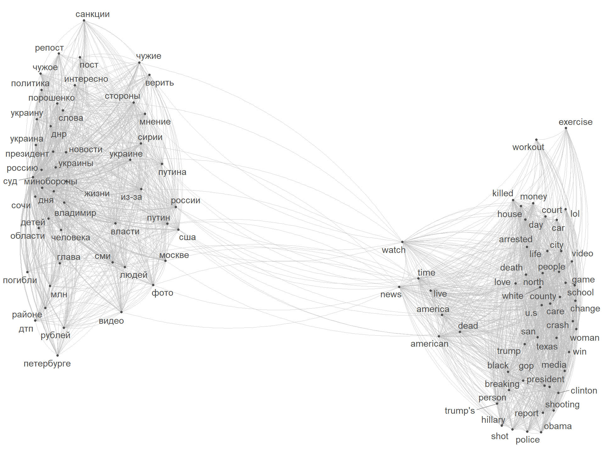
The two worlds collide on the topic of USA …
With the mightiness of Quanteda, we could do a lot of further exploratory analysis and so on… However, it’s really about time to focus on a smaller and language-specific subset, as the following task (to be addressed in part #3 of this series) will be even more intense in terms of computing power and memory usage.
However, here’s a preview from Topic Modelling on the English-language subset (~2M Tweets):
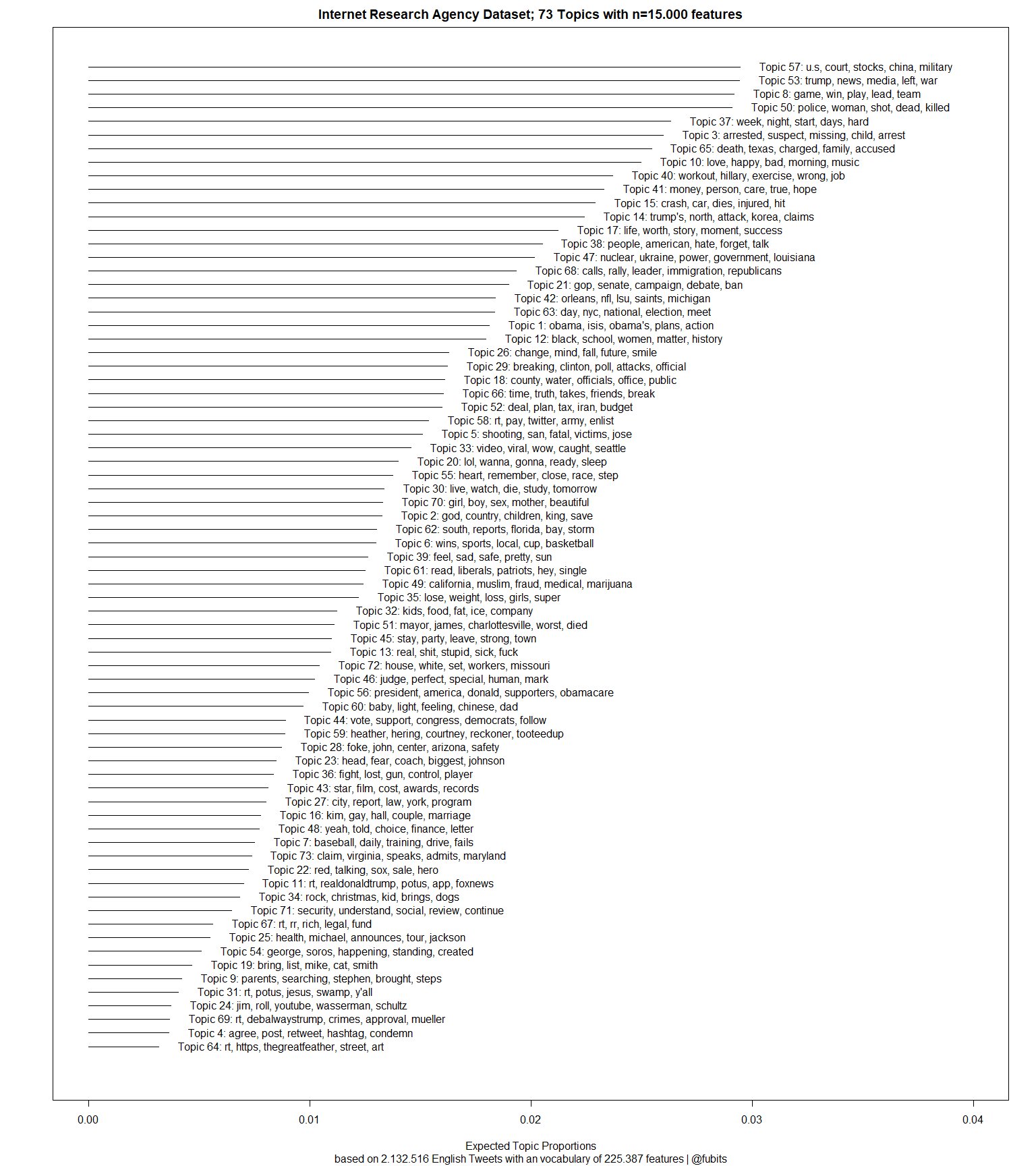
(73 Topics from 2M English-language Tweets; modelled with the stm()-package; K auto-induced with t-SNE/PCA)