[R] GIS like it's 2019: Pragmatic Workflows for Spatial Data, Pt. 1
Abstract / TL;DR
GIS with R is far beyond powerful. This is part 1 of a collection of up-to-date workflows for processing spatial data of all kinds with R. The collection involves sf, mapview, mapedit, osmdata, raster, stars, rnaturalearth and other packages combined with straight-forward recipes.
Update: added
mapdeck,leafgl, andtmapto the Tour d’Horizon
TL;DR: If you’re just here for the code / hacks, feel free to skip this intro and jump directly to the hands-on part.
1 A Bit of a Context: Spatial Tour d’Horizon
To be precise, my R “career” only started to gain traction when I was asked to create a low-budget CC0 print map by a colleague almost one and a half years ago. This particular use case gave me enough of an impression of the awesomeness of the Rstats / FOSS-minded community, the holistic potential of R re: all things data, and in particular the #GIStribe’s continuous efforts to make spatial processing with R accessible to everyone. What I did not know back then (among maaaaany other things) was that there had already existed a dual system of Base R and Tidy / Tidy-fied R - even for spatial…
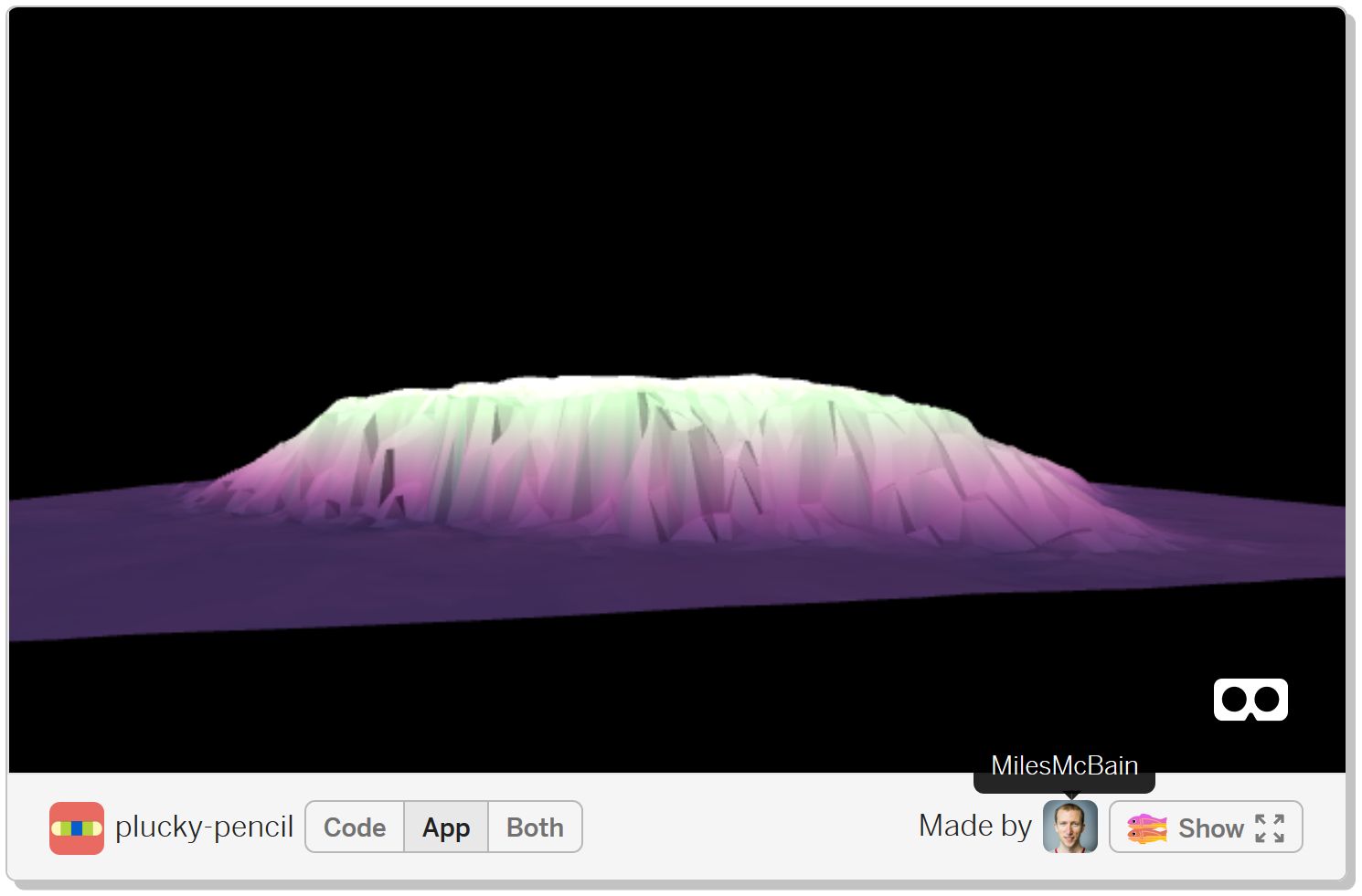
Screenshot of Miles McBain’s r2vr demo
If you consider that this post by @mdsumner was written already two years ago, and R users potentially have been able to do stuff such as to “colour a WebVR mesh by shading using a raster layer” (cf. screenshot above; McBain 2018) with the r2vr package in R for more than half a year now, I think this quote by Michael D. Sumner just perfectly sums up the status quo and the potential of “spatial / GIS with R” - just that this was two years ago…:
“GIS itself needs what we can already do in R, it’s not a target we are aspiring to[,] it’s the other way around.” (Sumner 2017)
I mean, this rayshader output (pictured below; click on the image to see the full GIF in action) by the package’s developer Tyler Morgan-Wall is not just a proof-of-concept. It’s out there on CRAN, it’s one technique already available for everyone with just a basic understanding of R and/or GIS.
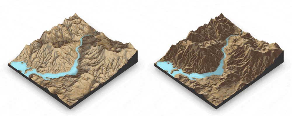
Screenshot of Tyler Morgan-Wall’s rayshader demo. Click this link to see the GIF in action.
Or have a look at what Michael D. Sumner has been working on with the quadmesh package, which will allow us - among other things - to take raster to another level. Same for Edzer Pebesma’sstars package with regards to its potential for tidy spatiotemporal data.
Update: @timsalabim3 and @ozjimbob reminded me of other prominent spatial packages I should have had mentioned here, but didn’t do so as I don’t have worked with them yet:
Ever heard of Uber’s {WebGL + Mapbox} based framework deck.gl for rendering really large datasets, XYZ data, and so on? @symbolixAU has you covered with the mapdeck package for R:
Mapdeck madness! Courtesy of SymbolixAU/mapdeck.
Prefer Leafletover Mapbox but still need to display 100K+ points on a map? @timsalabim3 / Team r-spatial have ported something for ya’:
And if you need to make thematic maps and/or don’t want to plot your spatial objects with ggplot, have a look at Martijn Tennekes’s tmap, which is also very well covered by Lovelace/Nowosad/Muenchow 2018, and gives you a lot with very few lines:
# from tmap vignette
# https://cran.r-project.org/web/packages/tmap/vignettes/tmap-changes-v2.html#tm_tiles
library(tmap)
data(World, metro)
tmap_mode("view")

tm_basemap(leaflet::providers$CartoDB.PositronNoLabels, group = "CartoDB basemap") +
tm_shape(World) +
    tm_polygons("HPI", group = "Countries") +
tm_tiles(leaflet::providers$CartoDB.PositronOnlyLabels, group = "CartoDB labels") +
tm_shape(metro) +
    tm_dots(col = "red", group = "Metropolitan areas") +
tm_view(set.view = 1)
In short, GIS with R is efficient, effective, affordable,
Shinyshiny, and complex enough to serve as the domain for showcasing R and as an exhaustive use case for new R users (or their supervisors). Let us look into that claim now.
2 Use Case
Recently, I did another but far more extensive freelance gig involving custom mapping of real-world geodata, and thereby discovered so many really helpful / effective / efficient / cool packages, methods, tools and workflows that I decided to write another GIS/mapping post. It’s simply time to give something back to the community (and to create a useful reference entry for my future self).
Update: The study on “The Logic of Chemical Weapons Use in Syria” has now been published during the Munich Security Conference 2019. It’s an acribic piece of research by Tobias Schneider and Theresa Lütkefend from the Berlin-based Global Public Policy Institute (GPPi). The study examines and explains the logic behind 336 chemical weapons attacks (98% by regime) during the Syrian Civil War. I had the challenging honour to help visualise the overall extent and the attack patterns in a few selected case studies:

Selected visuals from the “Nowhere to Hide” study on the use of Chemical Weapons in Syria. Read the full report on GPPi’s website. Almost all maps are CC-licensed.
All maps / visuals (including the spatial event data) where preprocessed and rendered with R and are based on vector data from Natural Earth and OpenStreetMap. Final polishing for print/pdf/web was done with Affinity Designer.
In this post, we’re going to take a tour through several versatile spatial packages for R. As a use case, we’re going to visualize cycling data from Berlin-based Tagesspiegel’s DDJ #radmesser-project for my hometown Berlin, Germany.
This post is not about basic geocomputation / GIS / cartography concepts. Regarding this, there already are plenty of excellent up-to-date resources such as Lovelace/Nowosad/Muenchow 2018, Jesse Adler’s solid series on R for Digital Humanities, or Sébastien Rochette’s Introduction to mapping with {sf} & Co..
Rather, this post is more of my own glossary for all the magical things / hacks.
If there’s a single really helpful thing to keep in mind for now, it’s this common basic representation of GIS’ data layers:
Source: National Coastal Data Development Centre (NCDDC), National Oceanic and Atmospheric Administration (NOAA), USA
3 Packages
These are the packages we’re going to use:
library(tidyverse)
library(sf)
library(mapview)
library(mapedit)
library(rnaturalearth)
library(osmdata)
# library(raster) # I prefer to use raster::fun() since raster::select() masks dplyr::select()
4 Basic Workflows - Vector
Let’s assume that we want to make some kind of a map, be it because we actually need a map (i.e. for a great book on European foreign policy), or maybe just to give some spatial data some kind of a cognitive canvas. As geodata tends to take up non-trivial amounts of resources (bandwidth, memory, CPU), it could be useful to focus on only a particular geographic extent. This is where I learned to love the concept of a bounding box (BBOX). Instead of literally downloading the whole world (thereby straining someone else’s bandwidth / server capacity) and then running costly query/filter operations, we can easily define bounds first.
If you’re spatially literate and therefore easily can spot whether you need Lat/Lon or Lon/Lat, or what projection / CRS your favourite BBOX-providing workflow offers, you probably can skip this and just define your BBOX manually with something like bbox <- c(xmin, ymin, xmax, ymax). I tend to struggle with this (even when using web tools such as http://bboxfinder.com), because I either mix up Lat/Lon or underestimate the spatial extent of my geodata or whatever. This is why I think that these three approaches below might be helpful to others, too.
4.1 Basemap Bounding Box: Three Approaches
So first of all we want to decide on the extent of the basemap. Since this is a recurrent task but with varying parameters, I’m offering three different approaches, based on
the bounding box (BBOX) of a spatial object (i.e. Admin 1 level Federal state|s)
the bounding box of spatial data (i.e. the geocoded cycling data)
a hand-drawn rectangle turned into a BBOX
4.1.1 Bounding Box: Object-based
Here, we start with our spatial object of reference. I prefer to work with Open Access / Public Domain data (and not Google Maps / Bing et al.), so let’s fetch some vector data from the Natural Earth project - but as class = Simple Feature instead of Esri’s proprietary (and less tidyverse-friendly) Shapefile format.
For your use case, consult the vignette for
rnaturaleath::ne_download()and the Natural Earth website. For the sake of resource efficiency I also recommend to download the data once and then to store it locally withsave/saveRDSfor future use. As I work a lot with Natural Earth data, I have mounted a network folderD:/GIS/with all the raster and vector data I’ve downloaded so far. However, I do not recommend downloading the “Download all X themes” files, since this gives you a) shapefiles instead of Simple Features, and b) UTF-8 encoding issues for the feature labels, depending on when the particular theme was compiled the last time.
Download a certain Natural Earth feature set (“theme”): world-wide substates / Admin-1 level
substates10 <- rnaturalearth::ne_download(scale = 10, type = "admin_1_states_provinces", category = "cultural", returnclass = "sf")

# saveRDS(substates10, file = str_c(here::here("static", "data", "GIS_workflows", "/"), "substates10.rds"))
# substates10 <- readRDS(file = str_c(here::here("static", "data", "GIS_workflows"), "/", "substates10.rds"))
Subset the Federal State of Berlin
berlin_sf <- substates10 %>% filter(name == "Berlin")Next, we’ll use the amazing sf package to fetch Berlin’s bounding box (BBOX).
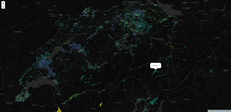
berlin_bbox <- sf::st_bbox(berlin_sf)So… wanna have a quick glimpse at Berlin’s bounding box? Here’s all that it takes with the game-changing mapview package by Tim Appelhans et al.:
berlin_bbox %>% mapview::mapview()Caveat: To keep memory and CPU load low for everyone browsing this post, I mostly will display the output of interactive widgets as
.jpg.
If you want to set the “CartoDB Dark Matter” basemap as your default (or any other of the themes supported by Leaflet ), you might want to add this setting to your
.Rprofile:
mapview::mapviewOptions(basemaps = c("CartoDB.DarkMatter", "CartoDB.Positron", "Esri.WorldImagery", "OpenStreetMap", "OpenTopoMap"))And since mapview() is just cool, we clan plot and inspect our Berlin object and the BBOX at the same time. For this we’re going to convert the BBOX object into a regular simple feature object with sf::st_as_sfc on the fly:
mapview::mapview(list(sf::st_as_sfc(berlin_bbox), berlin_sf))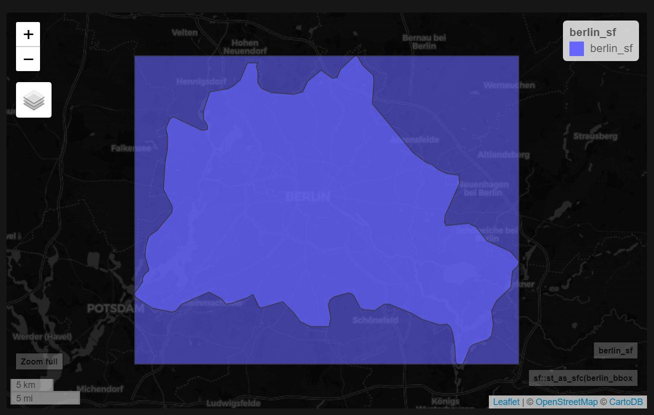
This box would probably be too narrow for further static editing (i.e. for a print map), so it would be cool if we could simply increase the BBOX’s extent. Since the coordinates in the bbox are stored as a numeric vector c(xmin, ymin, xmax, ymax), we can easily expand the bbox by providing another vector of length = 4 and see if the extent is better on the fly:
(berlin_bbox + c(-0.1, -0.1, 0.1, 0.1)) %>%
  # sf::st_as_sfc() %>%
  mapview::mapview()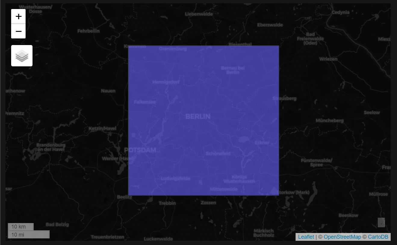
That seems generous enough. So let’s preserve this box for later.
berlin_bbox <- berlin_bbox + c(-0.1, -0.1, 0.1, 0.1)4.1.2 BBOX from data
Another approach to get a reasonable bounding box is to calculate the BBOX based on your geodata.
As mentioned above, I’m going to use the freshly released cycling data from the Berlin-based Tagespiegel DDJ / Innovation Lab for the final use case. The data has been collected as part of the sensor-based #radmesser project, where Lab leader Hendrik Lehmann’s team of journalists and/or developers equipped 100 (!) cyclists with close-range sensors to measure the distance of passing-by cars and trucks on Berlin’s roads. Goal: Demonstrate the at-risk status of cyclists in Germany’s capital.
Make sure to check out the award-winning project’s website and the project’s repo.
It’s probably worth the remark that getting the data into R is as simple as sf::st_read(URL)…
# License: ODC-By v1.0/Tagesspiegel Radmesser/https://radmesser.de
# cf. https://github.com/tagesspiegel/radmesser/blob/master/opendata/LICENSE.md
berlin_bike <- sf::st_read("https://github.com/tagesspiegel/radmesser/blob/master/opendata/detailnetz_ueberholvorgaenge.geo.json?raw=true")

# saveRDS(berlin_bike, file = str_c(here::here("static", "data", "GIS_workflows", "/"), "berlin_bike.rds"))
# berlin_bike <- readRDS(file = str_c(here::here("static", "data", "GIS_workflows"), "/", "berlin_bike.rds"))
However, st_read silently drops the “stats” field (which is legit, since a GeoJSON feature is defined as
geometry + propertiesonly) which contains the single measurements. Or rather: I have no 1-liner idea how to preserve it, be it in QGIS, withjsonlite, or by transforming with http://geojson.io. Fortunately, the Radmesser-team also provides a CSV with the measurements and a column with the respective streets key. So we can address this later (in Pt. 2 of this series). FYI, this is what the structure of this GeoJSON file looks like, so feel free to hit me up on Twitter if you know a solution:
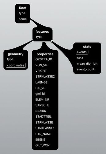
Help! How to preserve the stats field!?
Nonetheless, we can quickly have a look at the traced roads where the 15K+ individual measurements where taken, and also visualize the road class with zcol = "variable".
mapview::mapview(berlin_bike, zcol ="STRKLASSE1")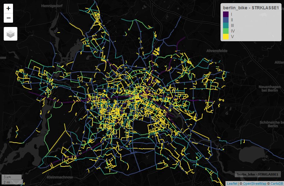
And now the data-based BBOX:
berlin_bike_bbox <- sf::st_bbox(berlin_bike)mapview::mapview(list(st_as_sfc(berlin_bike_bbox), berlin_bike))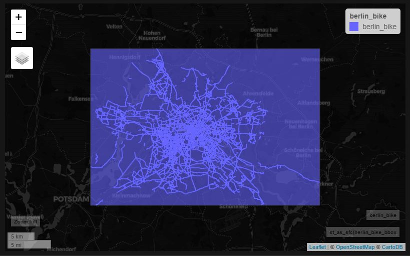
Easy, right?
4.1.3 Hand-drawn BBOX with mapedit
If neither the feature/object-based nor the geodata-based BBOX is sufficient for you (i.e. because you need a custom extent not matching the data), we can literally draw the box with the super-handy mapedit package. For this, we’ll take the cycling data just to add some context, and then will interactively draw a rectangle polygon and store the output in new object.
Don’t forget to click the “Done” button to finish editing.
(berlin_custom <- mapview::mapview(berlin_bike) %>% mapedit::drawFeatures())

# saveRDS(berlin_custom, file = str_c(here::here("static", "data", "GIS_workflows", "/"), "berlin_custom.rds"))
# berlin_custom <- readRDS(file = str_c(here::here("static", "data", "GIS_workflows"), "/", "berlin_custom.rds"))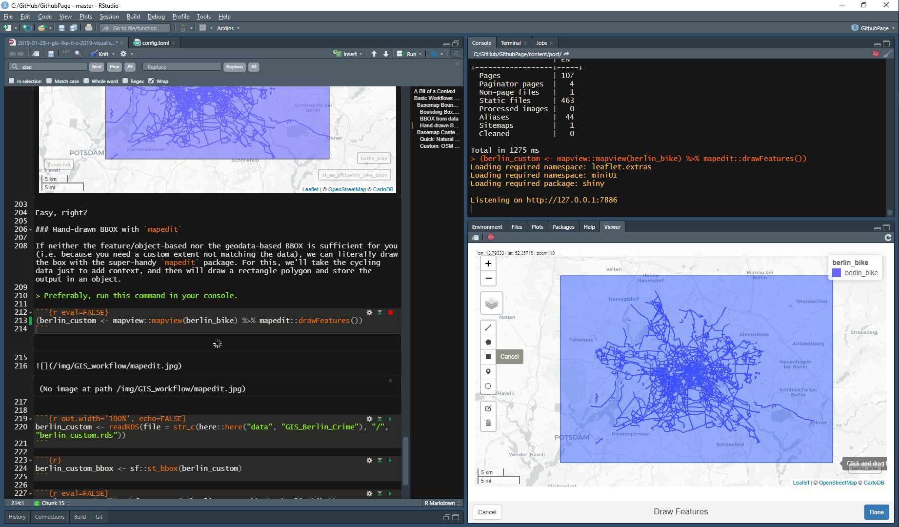
The resulting object is not a BBOX, obviously, but we can just fetch the object’s BBOX, and voila - habemus BBOX.
berlin_custom_bbox <- sf::st_bbox(berlin_custom)Let’s double-check our custom BBOX with the cycling data and the Berlin feature object.
mapview::mapview(list(sf::st_as_sfc(berlin_custom_bbox), berlin_sf, berlin_bike))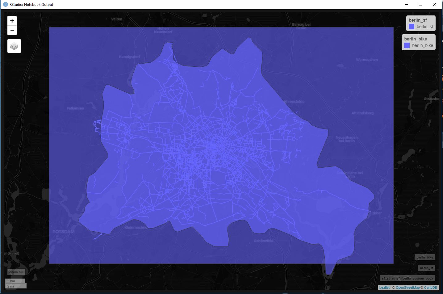
Dammit, I messed up the lower-right corner by omitting a piece of Berlin’s south-east (if the use case were to include all of Berlin). But we can easily re-draw the box with mapedit or use the bbox <- bbox + vector hack from above.
berlin_custom_bbox## xmin ymin xmax ymax
## 13.02704 52.35716 13.79334 52.67722We’re after ymin in this case, so we could either do berlin_custom_bbox["ymin"] <- newValue or manipulate the value with berlin_custom_bbox["ymin"] - 0.1.
Ok, enough BBOXing for today. Next: How to get any vector data we want into R.
4.2 Basemap Contents
For creating a custom map / visualization you might want to have as much control of what’s displayed on the basemap level as possible. Depending on the resolution / zoom-level of your map, 1:10m vector data from Natural Earth might already be sufficient. For more detail and features (esp. to play around with when you have a certain Gestalt concept and/or want to map below regional level), querying OpenStreetMap data is probably the gold standard. We’ll look into both approaches in this Chapter.
4.2.1 Quick: Natural Earth
For the regional level, 1:10m vector data might already be sufficient. Let’s look at a Berlin map built from roads, rivers and lakes (and borders, of course). I’m going to load() the Natural Earth vector data from my local D:/GIS folder, but you could download everything as described above and below. Europe is privileged, so there’s supplemental data offered by Natural Earth for lakes and rivers (cf. Natural Earth: Rivers for more detail and licensing), so I’m going to use it here. However, the lakes data does not offer any objects in or around Berlin, so I’m sticking to the regular lakes data instead. For rivers, we get 3 results, but we might want to double-check with the base rivers data. Cause we can ;) And because inspecting your data before working with it is a core data science skill anyways - spatial or not.
But see for yourself:
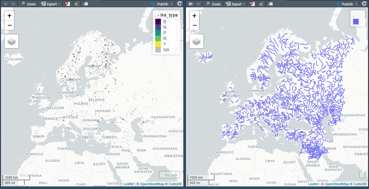
Supplemental data for European lakes (on the left) and rivers (on the right) from Natural Earth. Displayed with mapview of course!
So let’s fetch roads, lakes, and rivers from Natural Earth.
roads10 <- rnaturalearth::ne_download(scale = 10, type = "roads", category = "cultural", returnclass = "sf")

# basic lakes data
lakes10 <- rnaturalearth::ne_download(scale = 10, type = "lakes", category = "physical", returnclass = "sf")

# supplemental lakes data for Europe
# lakes10 <- rnaturalearth::ne_download(scale = 10, type = "lakes_europe", category = "physical", returnclass = "sf")
# saveRDS(lakes10, file = str_c(here::here("static", "data", "GIS_workflows", "/"), "lakes10_europe.rds"))
# lakes10 <- readRDS(file = str_c(here::here("static", "data", "GIS_workflows"), "/", "lakes10_europe.rds"))

# basic river data
rivers10_base <- rnaturalearth::ne_download(scale = 10, type = "rivers_lake_centerlines", category = "physical", returnclass = "sf")

# supplemental river data for Europe
rivers10_europe <- rnaturalearth::ne_download(scale = 10, type = "rivers_europe", category = "physical", returnclass = "sf")
# saveRDS(rivers10, file = str_c(here::here("static", "data", "GIS_workflows", "/"), "rivers10_europe.rds"))
# rivers10 <- readRDS(file = str_c(here::here("static", "data", "GIS_workflows"), "/", "rivers10_europe.rds"))
load("D:/GIS/vector/sf/roads10.RData")
load("D:/GIS/vector/sf/lakes10.RData")
load("D:/GIS/vector/sf/rivers10.RData")Now we’ll only pick those features which are needed aka are contained within our BBOX. There are a couple of approaches (i.e. by subsetting with a toponym, filtering by topological relation between two features (i.e. X within Y, intersects with), or the brute way of cropping with a BBOX).
But before we proceed, let’s inspect the lakes and rivers (base and Europe) objects, as we’re interested in finding out what we got:
mapview::mapview(list(rivers10_base, rivers10_europe, lakes10))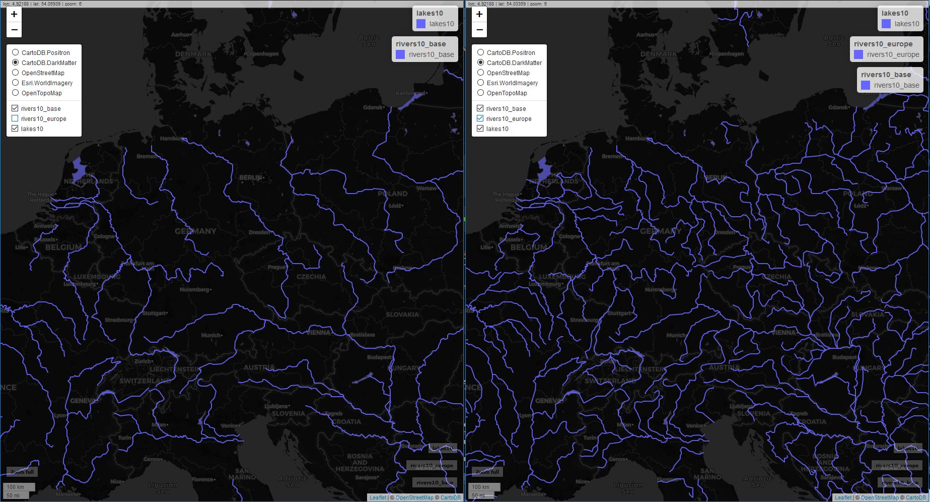
Comparison of base and supplemental data for rivers in Europe. Mapview is just awesome for this kind of exploratory tasks.
See how handy
mapview + sfis? We can visually compare two different sets of geometric features with the same easiness / usability and elegance as we do our usual exploratory data analysis of numeric data withsummary(),visdat,skimr,ggplot()and so on.
Anyways, we can see from our visual exploration that rivers10_base does not offer any rivers near or in Berlin. We can ignore this object.
Let’s look into subsetting the rest.
4.2.1.1 Subsetting by Toponym / Property
We did this already: We’ve subsetted the berlin_sf object from substates10 with filter(name == "Berlin"). That’s pretty straightforward if your data is clearly subsetable with an addressable object or explicit property (such as type = "highway"). However, that’s usually a bit trickier for cross-boarder features such as roads or rivers.
Deciding on whether to filter (or rather: query) or to crop depends on the size of the set you’re working with. And in practice, a combination of filter and crop is probably the most effective way. Our roads10 object contains 56K features, while lakes and rivers combined are around 3K. Even if 56K is not that much in 2019, you’ll still notice that it takes some time to compute the query (Big O calling!). If you have a dozen or so geometric objects to subset, you’ll quickly realize that size matters and that a clever query/crop/filter approach might save you resources.
Let’s look at sf::st_crop(), the mighty filter(sf::st_intersection()), and filter(sf::st_within()) which involves filtering lengths() > 0 and probably is not that intuitive when you’re new to GIS/spatial with R. At least that was the case for me.
4.2.1.2 Subsetting by Cropping: sf::st_crop
Cropping is straight-forward. We take our BBOX object (or any other feature from which st_crop can derive a BBOX) and then literally cut off all elements that extent beyond the BBOX.
lakes_berlin <- lakes10 %>% sf::st_crop(berlin_custom_bbox)
rivers_berlin <- rivers10_europe %>% sf::st_crop(berlin_custom_bbox)
Now we can simply use mapview or plot the resulting object with ggplot and geom_sf.
mapview::mapview(list(sf::st_as_sfc(berlin_custom_bbox), lakes_berlin, rivers_berlin))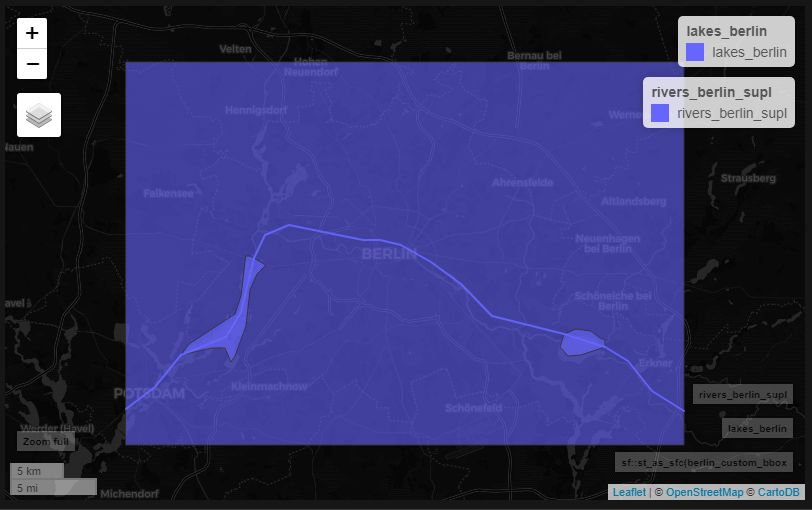
BBOX + cropped rivers and lakes
And now let’s plot the result with ggplot and berlin_sf as the background and use an equal-area projection for Berlin with crs = 3068 with is equivalent to crs = sf::st_crs(3068)
If you need a particular CRS for your use case, https://epsg.io/ might come in handy.
ggplot() +
  geom_sf(data = berlin_sf, fill = "lightgrey", color = "black") +
  geom_sf(data = lakes_berlin, fill = "blue") +
  geom_sf(data = rivers_berlin, aes(size = strokeweig), color = "blue") +
  geom_sf_label(data = rivers_berlin, aes(label = name)) +
  scale_size(range = c(0.5,2)) +
  theme_minimal() +
  guides(size = FALSE) +
  xlab("") +
  ylab("") +
  coord_sf(crs = 3068)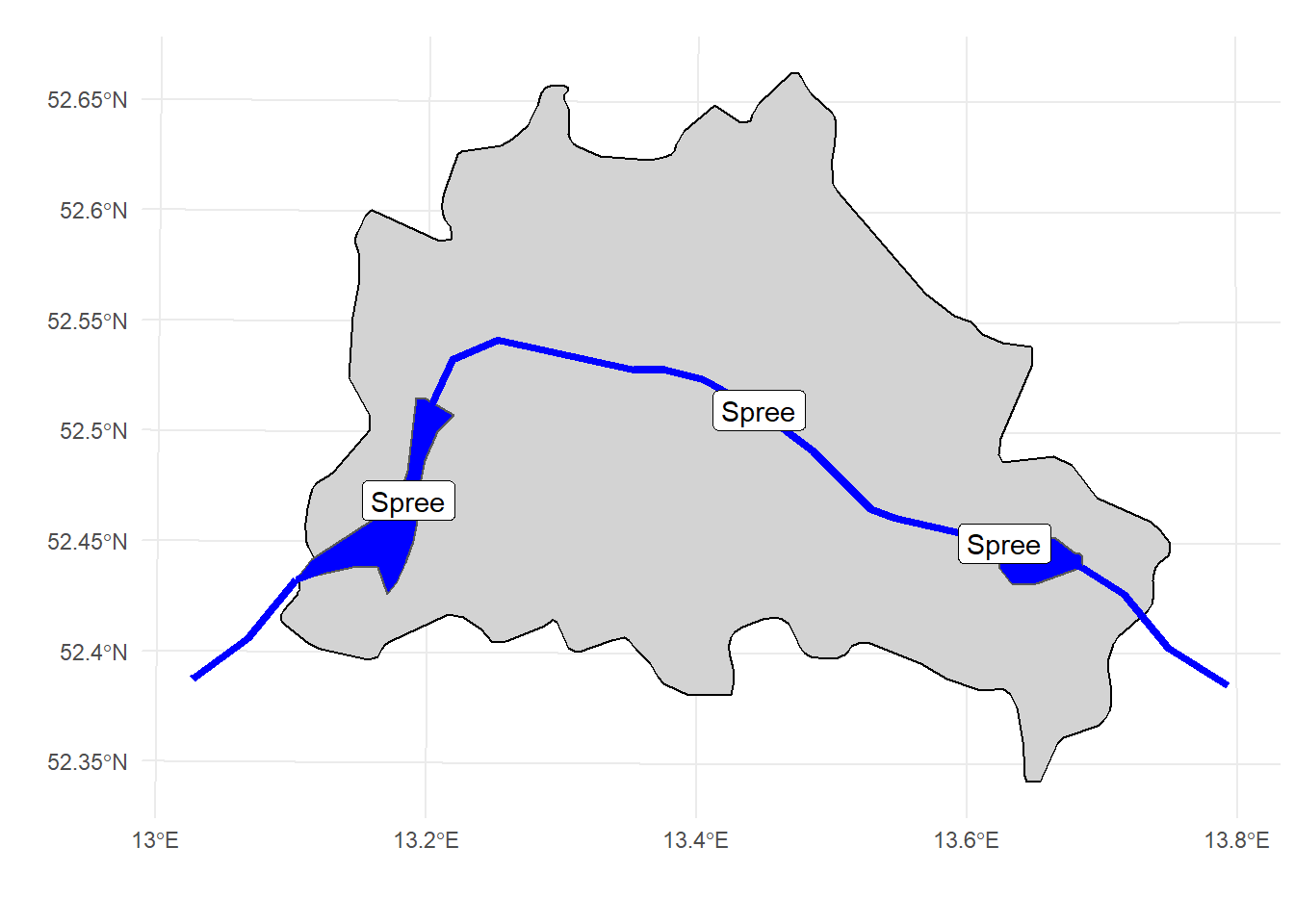
4.2.1.3 Subsetting by Topological Relation: sf::st_operation()
This is as accurate as it gets, but you might need to take some time to understand the basic set of geometric operations implemented in the sf() package. (Actually, I only understood sf::st_intersection while writing this paragraph… .) Just as a handy example, let’s say that we want to reduce our (world) roads10 object to Berlin’s shape. This a regular geocomputational operation, and we’re going to use sf::st_intersection(). Notice that this is a different kind of operation as sf::st_within(), which will be used next. st_intersection() returns a transformed object, while sf::st_within() is more of a binary query which returns TRUE/FALSE results, in the first place.
Since we already can assume that the result cannot extent beyond Berlin’s BBOX, we should first crop the (global) roads10 object with Berlin’s BBOX in order to reduce the computational cost of this operation.
roads_berlin_sf <- roads10 %>%
  sf::st_crop(berlin_custom_bbox) %>%
  sf::st_intersection(berlin_sf)
Here’s the result (and Kudos to Ryan Peek for using the Google-friendly “clip object to shape” lingo):
ggplot() +
  geom_sf(data = berlin_sf) +
  geom_sf(data = sf::st_as_sfc(berlin_custom_bbox), alpha = 0.3) +
  geom_sf(data = roads_berlin_sf, aes(color = type)) +
  theme_minimal() +
  coord_sf(expand = FALSE, clip = "on")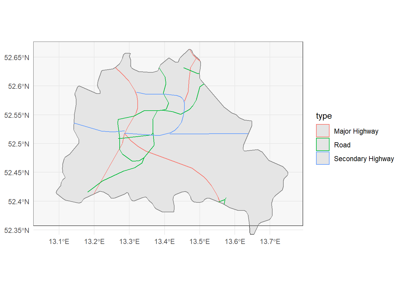
I guess it’s pretty obvious how powerful the sf package and ggplot's geom_sf() are. But let’s not forget about mapview()!
mapview::mapview(list(berlin_sf, roads_berlin_sf))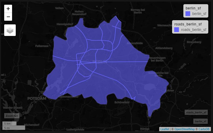
BBOX + cropped rivers and lakes
Now let’s look at sf::st_within() which calls for a different subsetting logic. The operation returns a binary predicate {0,1}, so we need to filter lengths() > 0. A bit tricky, right? Maybe it helps to read `sf``s Vignette.
In this example, we only want those roads, which are fully contained within Berlin’s border.
roads_berlin_sf <- roads10 %>%
  sf::st_crop(berlin_custom_bbox) %>%
  filter(lengths(st_within(., berlin_sf)) > 0)

ggplot() +
  geom_sf(data = berlin_sf) +
  geom_sf(data = sf::st_as_sfc(berlin_custom_bbox), alpha = 0.3) +
  geom_sf(data = roads_berlin_sf, aes(color = type)) +
  theme_minimal() +
  coord_sf(expand = FALSE, clip = "on")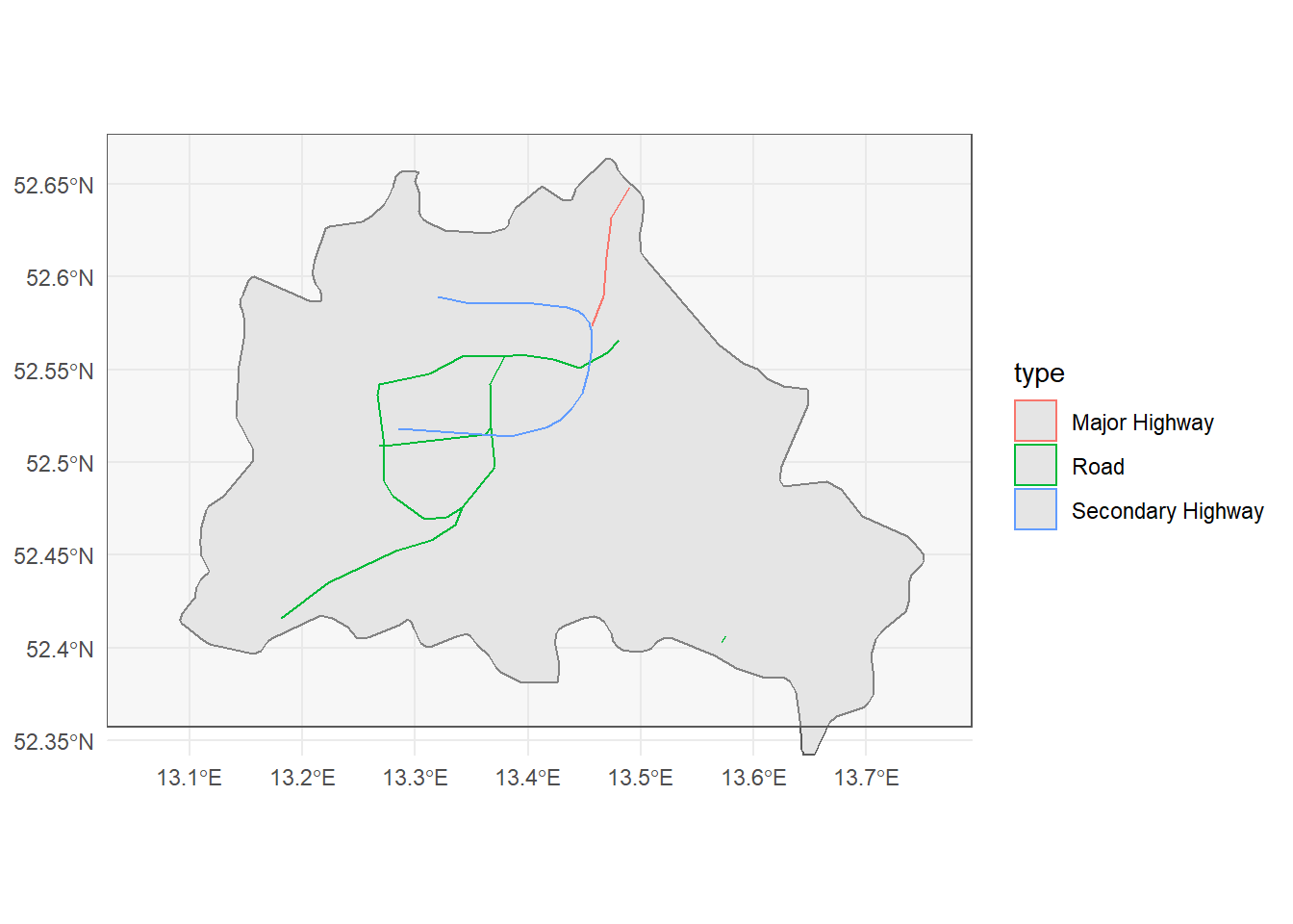
Of course, at this level of resolution the 1:10m data from Natural Earth does not offer enough granularity (i.e. to represent Berlin solely based on the signatures of Berlin’s roads). Let’s escalate with OpenStreetMap data.
4.2.2 Custom: OSM with osmdata (and all the above)
OpenStreetMap data is just a treasure trove for any mapper. It’s Open Data, it’s crowd-sourced by a huge community, and it’s granular even in the most exotic places. And this granularity exactly is a science in itself.
There are multiple non-developer ways to figure out how to get what you want, but all methods involve querying an OSM API (i.e. https://overpass-turbo.eu) for key=value assets such as highway=primary:
- https://taginfo.openstreetmap.org - quantified overview of all OSM key/value combinations
- https://www.openstreetmap.org - regular OSM front-end which includes a handy item picker tool if you struggle with ID’ing a particular object’s key/value pair
- https://overpass-turbo.eu - query from a front-end (incl. a wizard) and then to export as JSON and proceed with:
- https://mapshaper.org - turn the JSON layers in question into a condensed shapefile (and simplify the features with a GUI, if necessary)
Here’s a simple query as an example:
# berlin_osm_roads <- osmdata::opq(bbox = "berlin") %>% # alternative A
berlin_osm_roads <- osmdata::opq(bbox = berlin_bbox) %>% #  alternative B
  # osmdata::add_osm_feature(key = "highway") %>%
  osmdata::add_osm_feature(key = "highway", value = c("primary", "trunk", "motorway", "secondary", "tertiary")) %>%
  # osmdata::add_osm_feature(key = "highway", value = "primary") %>%
  osmdata::osmdata_sf()
# saveRDS(berlin_osm_roads, file = str_c(here::here("static", "data", "GIS_workflows", "/"), "berlin_osm_roads.rds"))
# berlin_osm_roads <- readRDS(file = str_c(here::here("static", "data", "GIS_workflows"), "/", "berlin_osm_roads.rds"))
The returning object is a bit messy (and huuuuge in-memory). It’s a list of lists of simple features (since we used osmdata::osmdata_sf())
berlin_osm_roads %>% names()## [1] "bbox" "overpass_call" "meta"
## [4] "osm_points" "osm_lines" "osm_polygons"
## [7] "osm_multilines" "osm_multipolygons"Don’t even bother to run
colnames(berlin_osm_roads$osm_lines)… G R A N U L A R I T Y
As we are interested in roads and our query only queried for roads (“highway”) as features, we should focus on osm_lines and osm_multilines.
berlin_osm_roads$osm_lines %>%
  count(highway) %>%
  arrange(desc(n)) %>%
  select(highway,n) %>%
  head(10)
## Simple feature collection with 10 features and 2 fields
## geometry type: MULTILINESTRING
## dimension: XY
## bbox: xmin: 12.96591 ymin: 52.21702 xmax: 13.90698 ymax: 52.77781
## epsg (SRID): 4326
## proj4string: +proj=longlat +datum=WGS84 +no_defs
## # A tibble: 10 x 3
## highway n geometry
## <fct> <int> <MULTILINESTRING [°]>
## 1 secondary 9653 ((13.83809 52.24558, 13.83934 52.24558, 13.84033 52.~
## 2 tertiary 5378 ((13.01489 52.24258, 13.01465 52.2425, 13.01425 52.2~
## 3 primary 3708 ((13.56098 52.25119, 13.56137 52.25107, 13.56169 52.~
## 4 motorway 1538 ((13.59075 52.24275, 13.59089 52.24227, 13.5911 52.2~
## 5 motorway_li~ 1180 ((13.58865 52.24389, 13.58903 52.2438, 13.58944 52.2~
## 6 trunk 518 ((13.25017 52.25944, 13.25085 52.25941, 13.25144 52.~
## 7 trunk_link 341 ((13.25252 52.25783, 13.25262 52.25775, 13.25274 52.~
## 8 secondary_l~ 178 ((13.35502 52.27282, 13.35517 52.27284, 13.35556 52.~
## 9 primary_link 153 ((13.60236 52.31128, 13.60252 52.31127), (13.36314 5~
## 10 tertiary_li~ 57 ((13.45458 52.29946, 13.45455 52.29964, 13.45457 52.~We’re talking about 13.5K road fragments here - and this is just road level 1 -3… That’s a bit different than Natural Earth 1:10m data.
berlin_osm_roads$osm_multilines %>% count(highway) %>% arrange(desc(n))## Simple feature collection with 2 features and 2 fields
## geometry type: MULTILINESTRING
## dimension: XY
## bbox: xmin: 13.1191 ymin: 52.45264 xmax: 13.50482 ymax: 52.529
## epsg (SRID): 4326
## proj4string: +proj=longlat +datum=WGS84 +no_defs
## # A tibble: 2 x 3
## highway n geometry
## <fct> <int> <MULTILINESTRING [°]>
## 1 primary 4 ((13.38425 52.45346, 13.38427 52.45337, 13.38436 52.4528~
## 2 secondary 3 ((13.43335 52.46403, 13.43357 52.46372, 13.43387 52.4633~berlin_osm_roads_crop <- berlin_osm_roads$osm_lines %>% sf::st_intersection(berlin_sf)
# berlin_osm_roads_crop2 <- berlin_osm_roads$osm_multilines %>% sf::st_intersection(., berlin_sf)Just to give you an idea: this is the level of granularity (and memory-intense granular vector data) we get:
plot(berlin_osm_roads_crop["highway"], key.pos = NULL)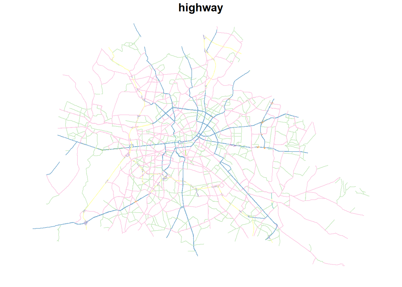
Or plotted with ggplot:
ggplot() +
  geom_sf(data = berlin_osm_roads_crop, aes(color = highway)) +
  # scale_size_discrete(c(0.1,2)) +
  coord_sf(datum = NA) +
  ggthemes::theme_map() +
  guides(color = FALSE)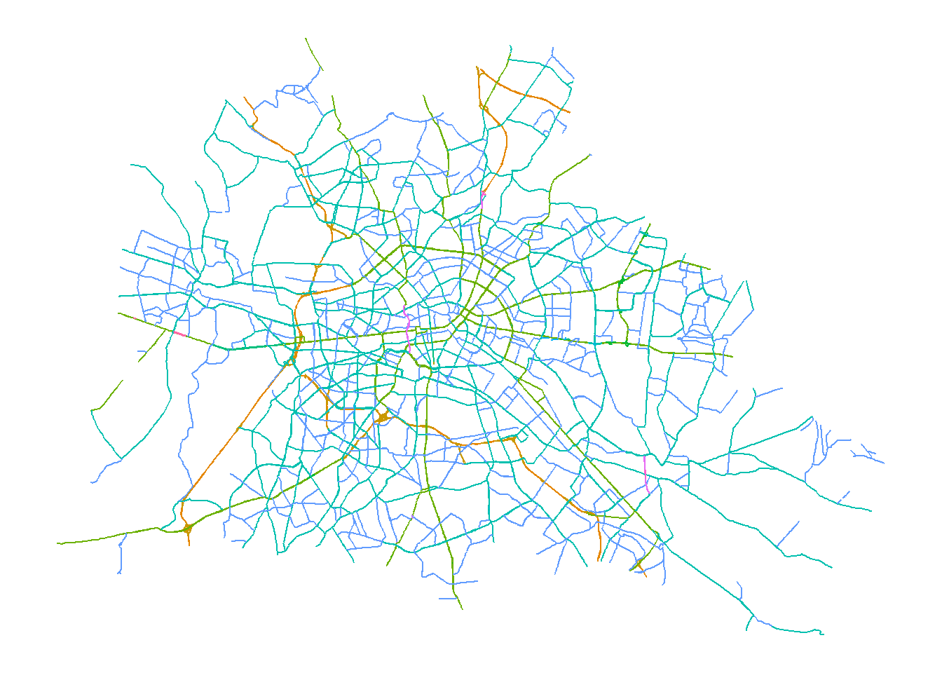
To be continued (
GeoJSON; Raster)…