2.1 Packages

knitr::opts_chunk$set(echo = TRUE)
library(tidyverse)
library(ggrepel)
library(maps)
library(ggthemes)
library(rasterVis)
library(maptools)
library(sp)
library(here)
# library(rnaturalearth) # <- source for geodata, but pkg masks some needed fun() from other packages, so rather address methods by rnaturalearth::fun() 

2.2 Geodata: World Map Data from Natural Earth

“Natural Earth is a public domain map dataset available at 1:10m, 1:50m, and 1:110 million scales. Featuring tightly integrated vector and raster data, with Natural Earth you can make a variety of visually pleasing, well-crafted maps with cartography or GIS software.” (Natural Earth)

Base Map (Admin-0 Level)

Let’s first import the geodata and check the basemap.

world <- rnaturalearth::countries110
plot(world)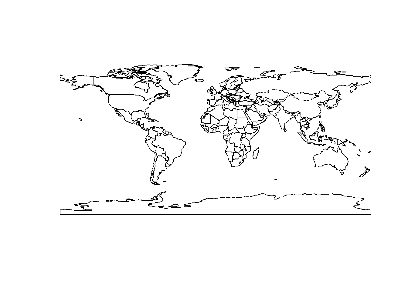

Ugh, not so pretty, right? But you have to start somewhere…

Spoiler: Some Geo-Objects – which were only mentioned later on – are missing at Admin-0 level.

-> Fetch Non-Admin-0 Elements (Guam & Singapore)

# countries10 <- rnaturalearth::ne_download(scale = 10,
#                                           type = 'countries',
#                                           category = 'cultural')
# save(countries10, file = "GIS_NPO_Data/countries10.rda")
data_path <- here("data", "GIS_NPO_Data", "/")
load(str_c(data_path, "countries10.rda"))

Where’s Guam?

# First, let's search for Guam:
# "Guam" %in% rnaturalearth::countries110$SOVEREIGNT #> FALSE, not "souvereign"
# Let's search below Admin-0 level within rnaturalearth::ne_states() 
# world.sub <- rnaturalearth::ne_states()
# head(world.sub, 1) # > either $name or $geounit
# "Guam" %in% world.sub$geonunit #> TRUE (vs. $name <- might be cruical for some)
Guam <- rnaturalearth::ne_states(geounit = 'guam')
Guam$category <- "D" # 4 regions A-D, as requested by colleague
plot(Guam)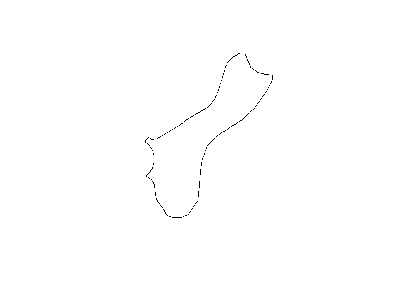

Where’s Singapore?

#> "Singapore" %in% rnaturalearth::countries110$SOVEREIGNT is FALSE, so apparently,
# it is a souvereign state, but as a city-state too *granular* for the 1:110m data.
#
# Let's have a look in the 1:10m data

Singapore <- countries10[countries10$SOVEREIGNT == 'Singapore',]
# "Singapore" %in% world.sub$geonunit #> is also TRUE, while
# "Guam" %in% countries10$SOVEREIGNT is FALSE
# Caution: Scope of data from countries110 & countries10 might differ!
Singapore$category <- "C"
plot(Singapore)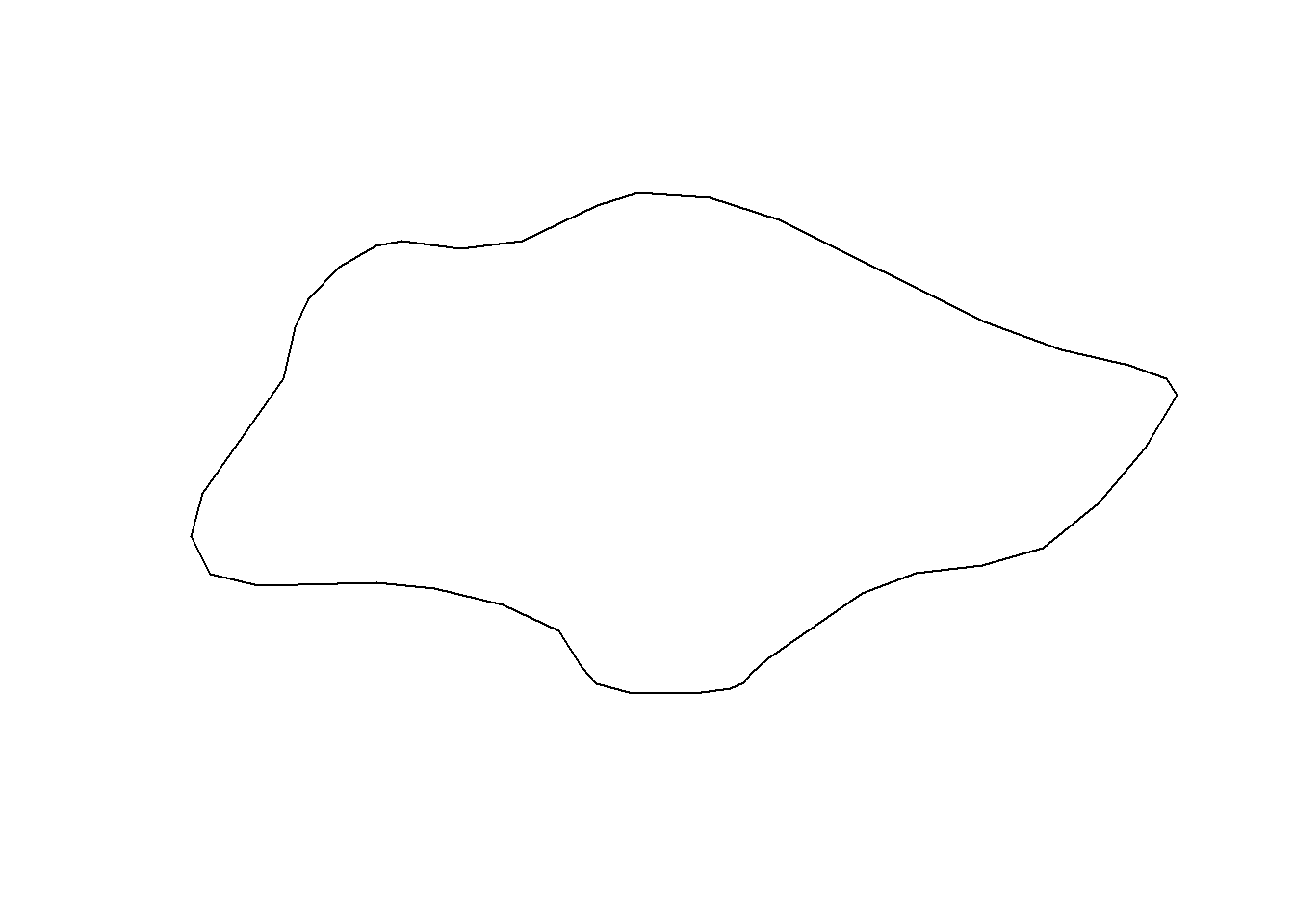

2.3 Assemble the Regions

China

asia_china <- world[world$sovereignt == 'China',]
asia_china$category <- "A"
plot(asia_china)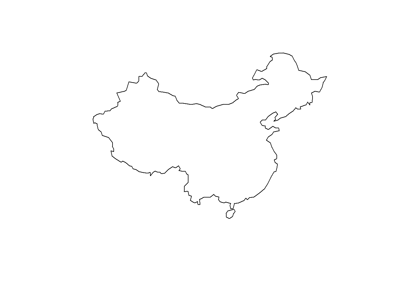

Eastern Asia (== $subregion minus China & Mongolia )

asia_east <- world[world$subregion == 'Eastern Asia' &
                     world$sovereignt != 'Mongolia' &
                     world$sovereignt != 'China',]
asia_east$category <- "D"
plot(asia_east)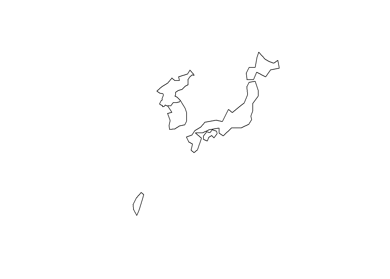

South-Eastern Asia

asia_seast <- world[world$subregion == 'South-Eastern Asia',]
asia_seast$category <- "C"
plot(asia_seast)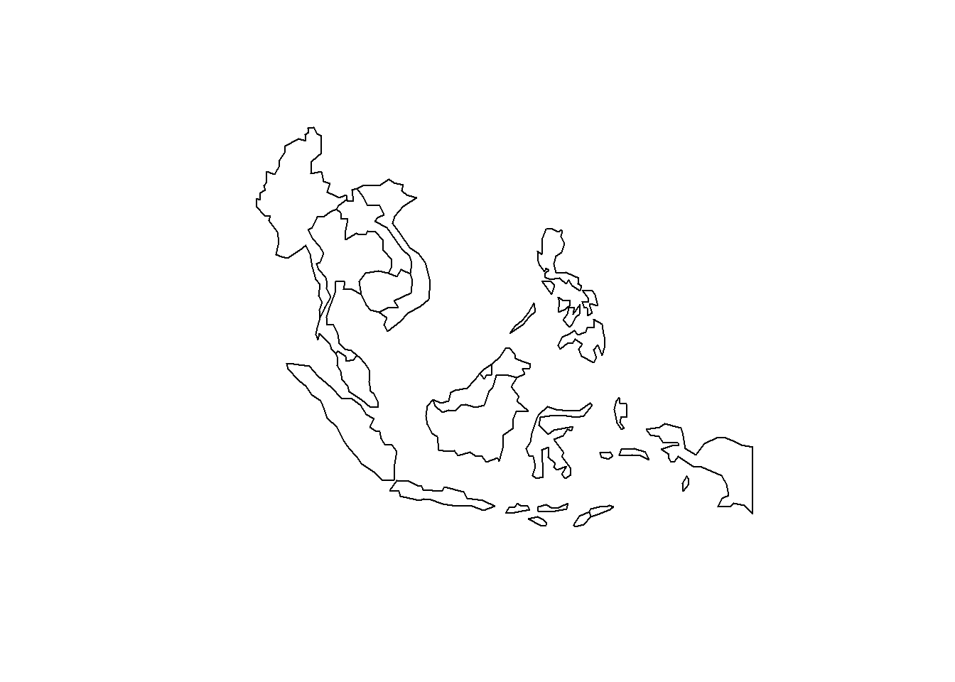

Central and South Asia (plus Russia & Mongolia)

asia_censouth <- world[world$region_wb == 'South Asia' |
                         world$subregion == 'Central Asia' |
                         world$sovereignt == 'Mongolia' |
                         world$sovereignt == 'Russia',]
asia_censouth$category <- "B"
plot(asia_censouth)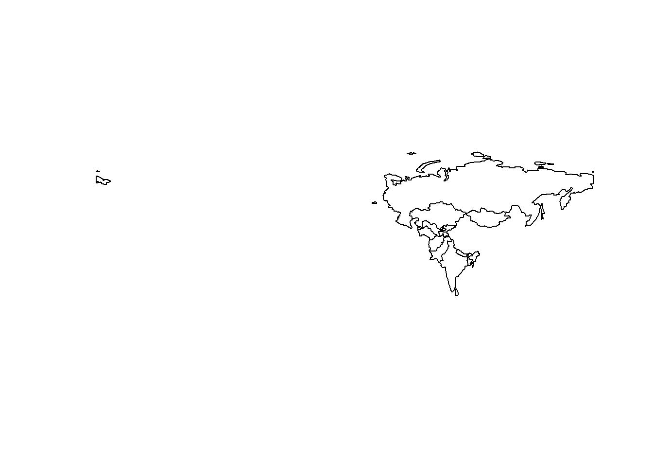

Why Russia, why? (cf. Thread & Solution for QGIS by Haluka )

Solution: Set left BBOX-Border to clip off Russia’s overlapping Tail

leftBorder <- 25
asia_censouth@bbox[1] <- leftBorder
plot(asia_censouth)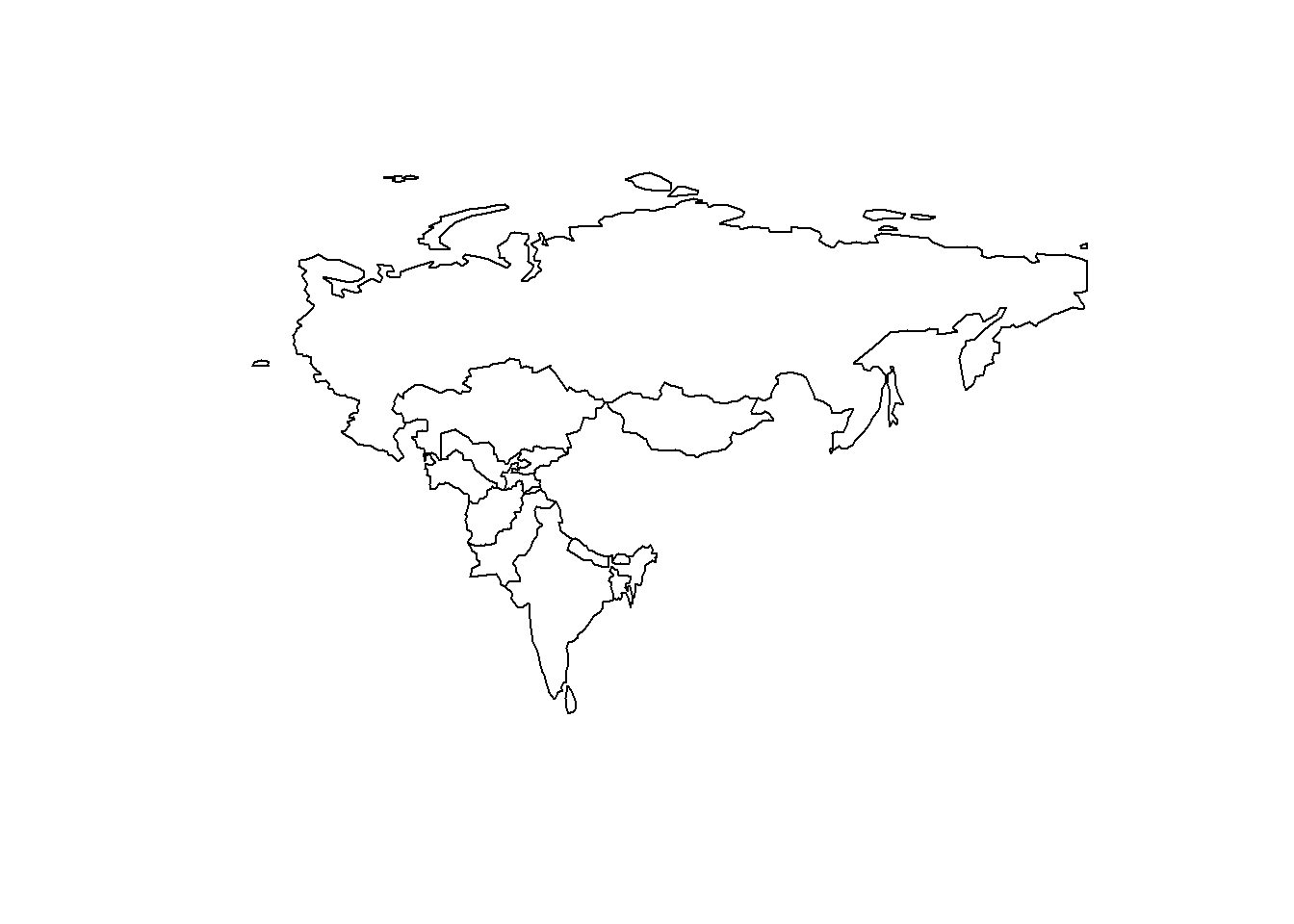

Consolidate the Core

asia_core <-  spRbind(
                spRbind(
                  spRbind(asia_china, asia_east),
                     asia_seast),
                        asia_censouth) # or just %>% next time :)
asia_core@bbox[1] <- leftBorder
plot(asia_core)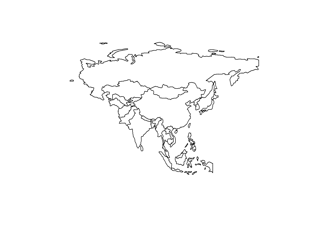

Consolidate the Rest

(Preview)

asia_rest <- world[world$region_un == "Asia" &
                     world$sovereignt != 'China' | 
                     world$region_un == "Oceania" | 
                     world$region_un == "Africa" |
                     world$region_un == "Europe",]
asia_rest@bbox[1] <- leftBorder
plot(asia_rest)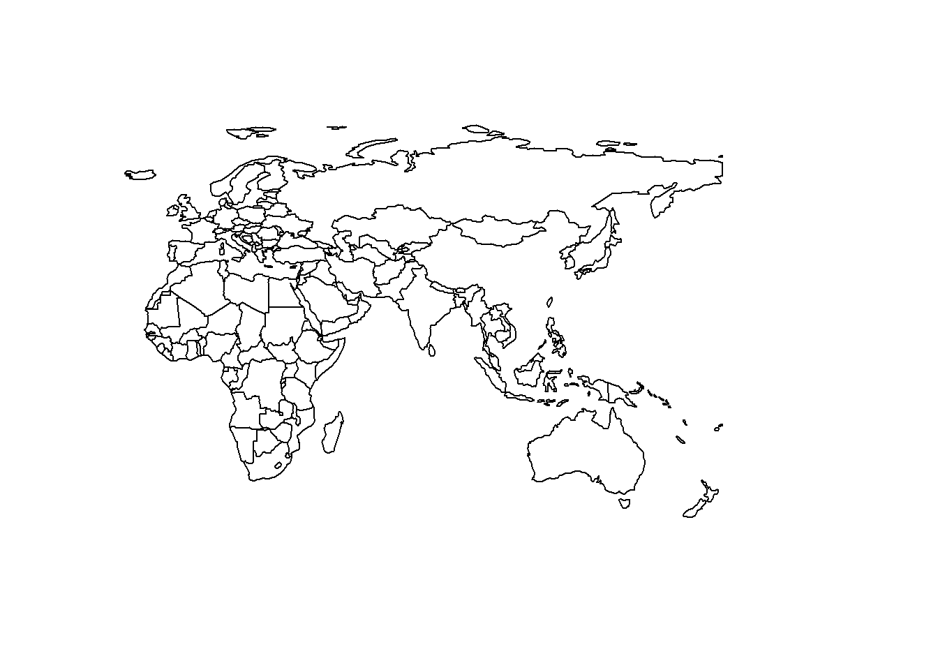

Remove the Core

asia_rest <- subset.data.frame(asia_rest,
                              !(asia_rest$sovereignt %in% asia_core$sovereignt))
asia_rest@bbox[1] <- leftBorder
plot(asia_rest)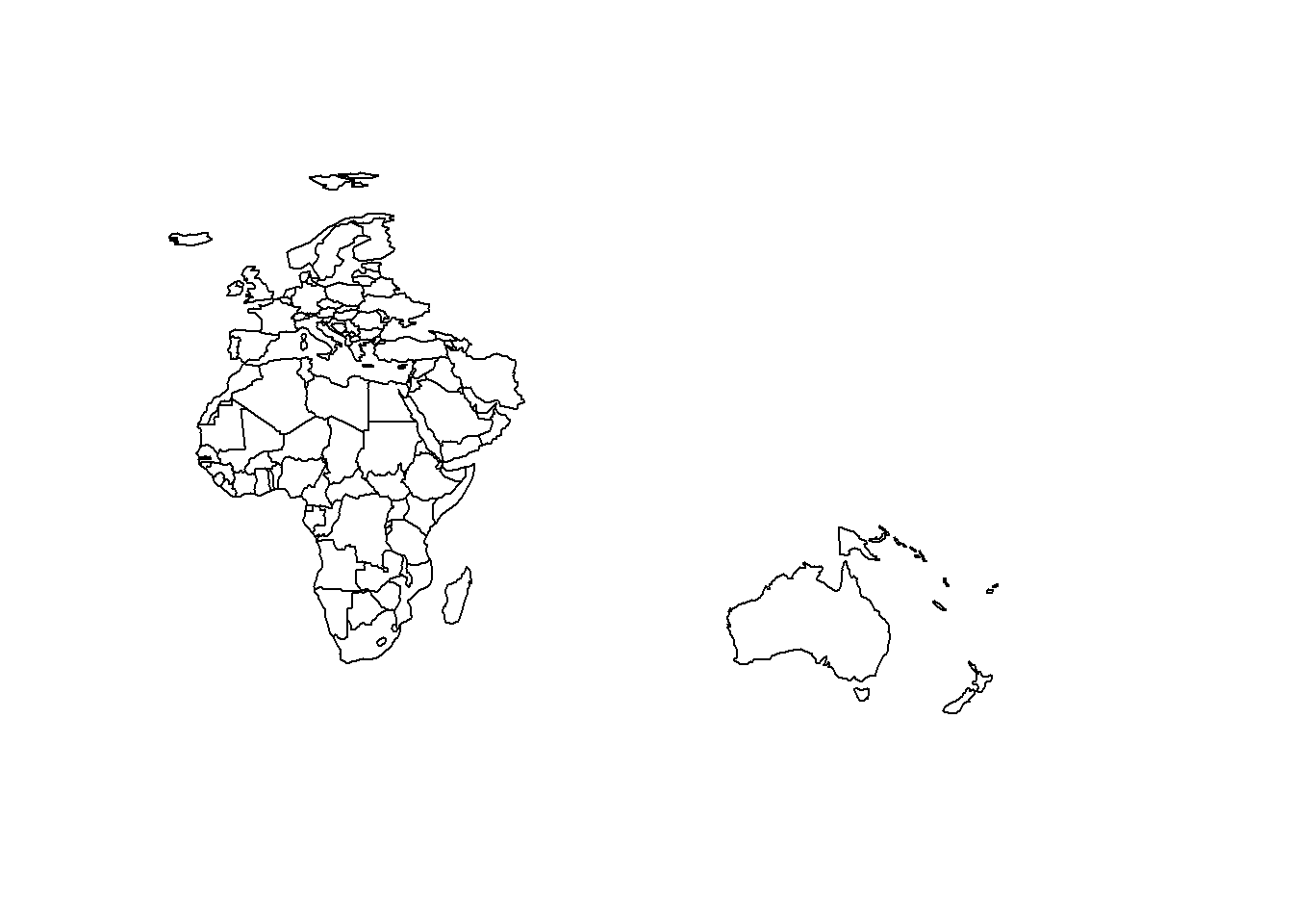

2.4 Convert Spatial Dataframe to Tidy Dataframe

(This was done before geom_sf / ggsf were introduced to ggplot2. There might exist a far more efficient solution right now, esp. with ggplot2.)

2019 Update: There exists a far more efficient solution, esp. with {sf, mapview, geom_sf, ... }

Tidy the Vector Data

asia_core@data$id <- row.names(asia_core@data)
Singapore@data$id <- row.names(Singapore@data)
Guam@data$id <- row.names(Guam@data)
asia_main <- broom::tidy(asia_core)
asia_main <- dplyr::left_join(asia_main, asia_core@data, by = 'id')
head(asia_main, 1)

## # A tibble: 1 x 71
##    long   lat order hole  piece group id    scalerank featurecla labelrank
##   <dbl> <dbl> <int> <lgl> <chr> <chr> <chr>     <int> <chr>          <dbl>
## 1  128.  49.8     1 FALSE 1     30.1  30            1 Admin-0 c~         2
## # ... with 61 more variables: sovereignt <chr>, sov_a3 <chr>,
## #   adm0_dif <dbl>, level <dbl>, type <chr>, admin <chr>, adm0_a3 <chr>,
## #   geou_dif <dbl>, geounit <chr>, gu_a3 <chr>, su_dif <dbl>,
## #   subunit <chr>, su_a3 <chr>, brk_diff <dbl>, name <chr>,
## #   name_long <chr>, brk_a3 <chr>, brk_name <chr>, brk_group <chr>,
## #   abbrev <chr>, postal <chr>, formal_en <chr>, formal_fr <chr>,
## #   note_adm0 <chr>, note_brk <chr>, name_sort <chr>, name_alt <chr>,
## #   mapcolor7 <dbl>, mapcolor8 <dbl>, mapcolor9 <dbl>, mapcolor13 <dbl>,
## #   pop_est <dbl>, gdp_md_est <dbl>, pop_year <dbl>, lastcensus <dbl>,
## #   gdp_year <dbl>, economy <chr>, income_grp <chr>, wikipedia <dbl>,
## #   fips_10 <chr>, iso_a2 <chr>, iso_a3 <chr>, iso_n3 <chr>, un_a3 <chr>,
## #   wb_a2 <chr>, wb_a3 <chr>, woe_id <dbl>, adm0_a3_is <chr>,
## #   adm0_a3_us <chr>, adm0_a3_un <dbl>, adm0_a3_wb <dbl>, continent <chr>,
## #   region_un <chr>, subregion <chr>, region_wb <chr>, name_len <dbl>,
## #   long_len <dbl>, abbrev_len <dbl>, tiny <dbl>, homepart <dbl>,
## #   category <chr>

Create centered Country Labels

centroids_df <- as.data.frame(coordinates(asia_core)) # returns centered points
centroids_df$sovereignt <- asia_core$sovereignt # add country names

# I had to include Guam and Singapore only after I already rendered the core
# map, so this is my rather awkward work-around to include them subsequently
sing_centroids_df <- as.data.frame(coordinates(Singapore))
sing_centroids_df$sovereignt <- Singapore$SOVEREIGNT
centroids_df <- rbind(centroids_df, sing_centroids_df)
Guam_centroids_df <- as.data.frame(coordinates(Guam))
Guam_centroids_df$sovereignt <- Guam$name
centroids_df <- rbind(centroids_df, Guam_centroids_df)

# rename the colnames
names(centroids_df) <- c("Long", "Lat", "Name")
head(centroids_df, 1)

##        Long      Lat  Name
## 30 103.8654 36.60943 China

2.5 Relief Raster

Get the Relief Raster File

# Either:
# physics <- rnaturalearth::ne_download(scale = 50, category = 'raster',
#                                       type = 'NE2_50M_SR_W', load = TRUE)

# OR:
# Download from: http://www.naturalearthdata.com/downloads/50m-raster-data/
# Here: NE2, shaded relief, water: http://www.naturalearthdata.com/http//www.naturalearthdata.com/download/50m/raster/NE2_50M_SR_W.zip
relief_world <- raster(str_c(data_path, "NE2_50M_SR_W.tif")) # 170 MB file
plot(relief_world)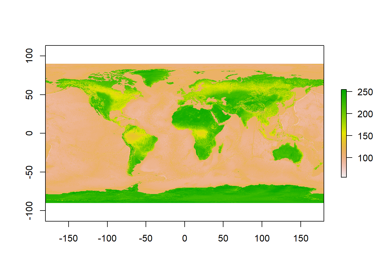

(If needed: reduce Raster Resolution)

# reduce resolution by 50% (I didn't do it since we want high-res for print)
# s2 <- aggregate(s, fact = 2)
# plot(s2)

Crop the Raster File

# deprecated:
# manually select the box for the region with mouse pointer -> quick but bad!!!
# s <- raster::select(relief)
# plot(s)

# OR:
# Crop around dataframe
# relief_sub <- crop(relief, extent(asia_rest))

# OR
# Clean & easy: just define the extend of the box
box <- extent(25, 155, -25, 60) # how to calculate ratio (i.e. 1: 1,48)?
relief_boxcrop <- crop(relief_world, box)
plot(relief_boxcrop)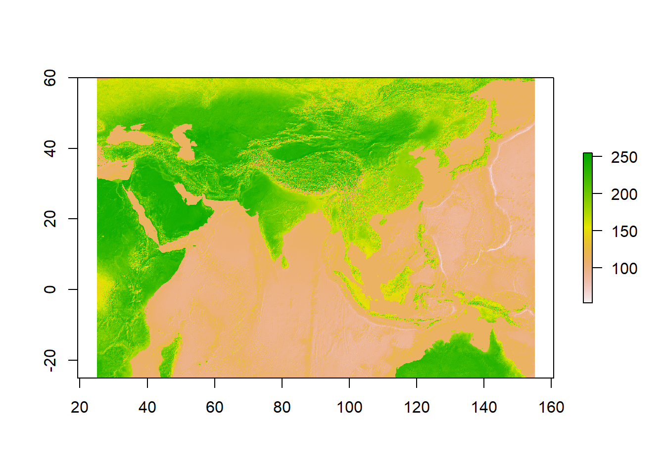

Raster for the Core Regions

# Mask everything apart from the core regions terrain
# relief_land <- raster::mask(relief_boxcrop, asia_core) # mask {E} != asia_core
# save(relief_land, file = "../../data/GIS_NPO_Data/relief_land.rda")
load(str_c(data_path, "relief_land.rda"))
plot(relief_land)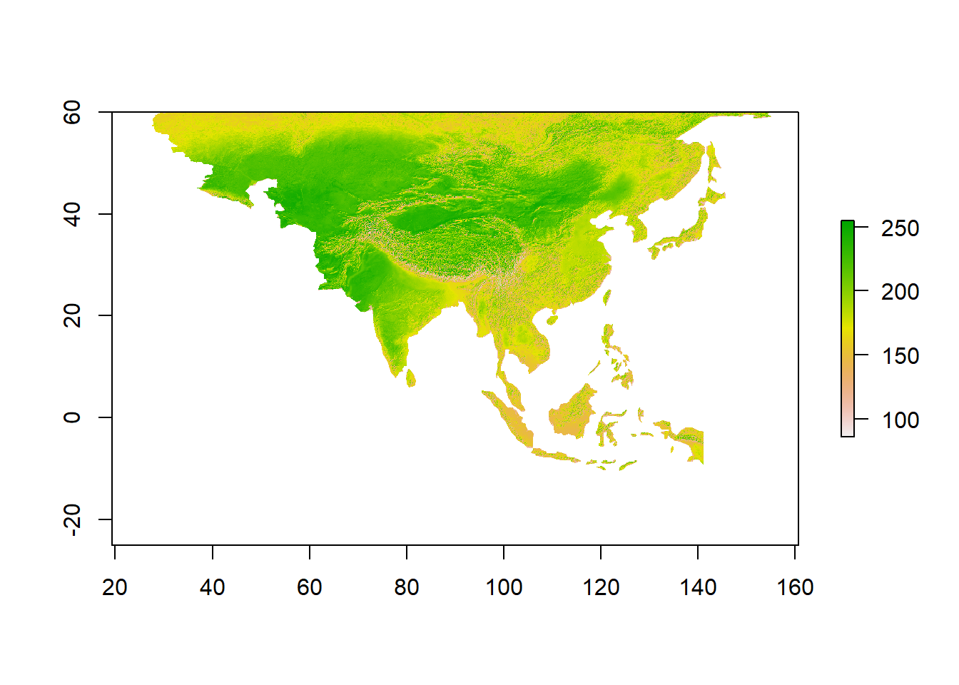

Convert Core Raster to SPDF to DF

# Raster to SPDF
relief_land_spdf <- as(relief_land, "SpatialPixelsDataFrame")
# SPDF to DF (for ggplot)
relief_land_df <- as.data.frame(relief_land_spdf) %>% 
  rename(value = `NE2_50M_SR_W`)
head(relief_land_df, 1)

##   value     x        y
## 1   113 29.05 59.98333

Raster for the Rest (Water & Terrain)

# relief_meer <- raster::mask(relief_boxcrop, asia_core, inverse=TRUE) # maskiert alles == asia_core
# save(relief_meer, file = "../../data/GIS_NPO_Data/relief_meer.rda")
load(str_c(data_path, "relief_meer.rda"))
plot(relief_meer)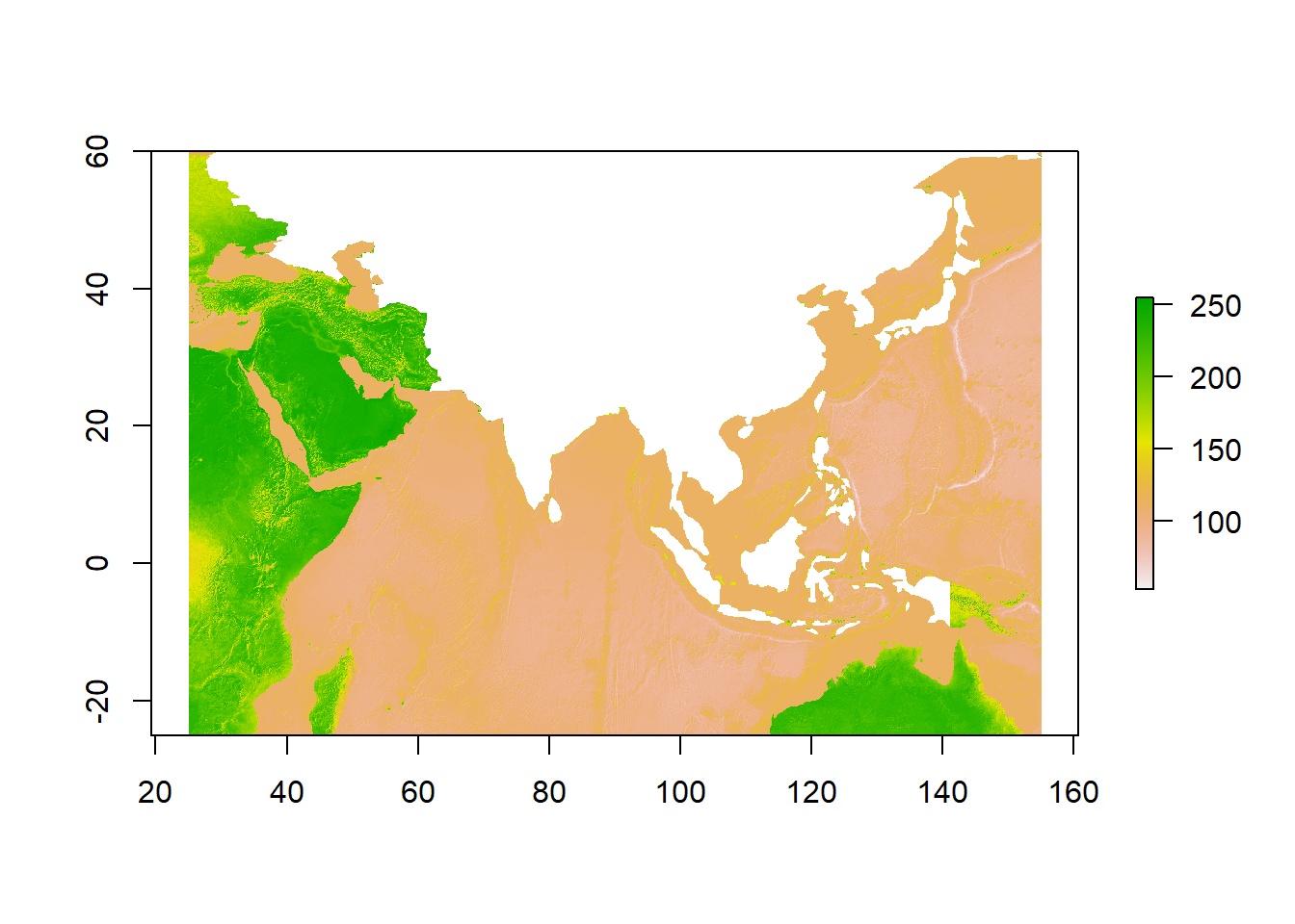

Convert 2nd Raster to DF

relief_meer_spdf <- as(relief_meer, "SpatialPixelsDataFrame")
relief_meer_df <- as.data.frame(relief_meer_spdf) %>% 
  rename(value = `NE2_50M_SR_W`)
head(relief_meer_df, 1)

##   value        x        y
## 1   112 25.01667 59.98333

3.1 Preview with Default Colors

ggplot() +
  # Polygons for the 4 regions
  geom_polygon(data = fortify(asia_main), alpha = 0.5,
               aes(x = long, y = lat, group = group,
                   fill = asia_main$category),
               color = "white", size = 1) +
  geom_polygon(data = fortify(asia_rest), alpha = 0.5,
               aes(x = long, y = lat, group = group),
               fill = "grey89", color = "white", size = 1) +
  geom_polygon(data = fortify(Singapore), alpha = 0.5,
               aes(x = long, y = lat, group = group),
               color = "white", fill = "red", size = 1) +
  geom_polygon(data = fortify(Guam), alpha = 0.5,
               aes(x = long, y = lat, group = group),
               color = "white", fill = "red", size = 1) +
  # normalise coordinates and crop canvas
  coord_equal(ratio = 1, xlim = c(25, 149), ylim = c(54.9, -25)) + # cropped
  theme_map() +
  theme(legend.position = "none") +
  # repel =  no overlapping between labels
  geom_text_repel(data = fortify(centroids_df),
                aes(label = Name, size = 12, x = Long, y = Lat),
                segment.colour = NA)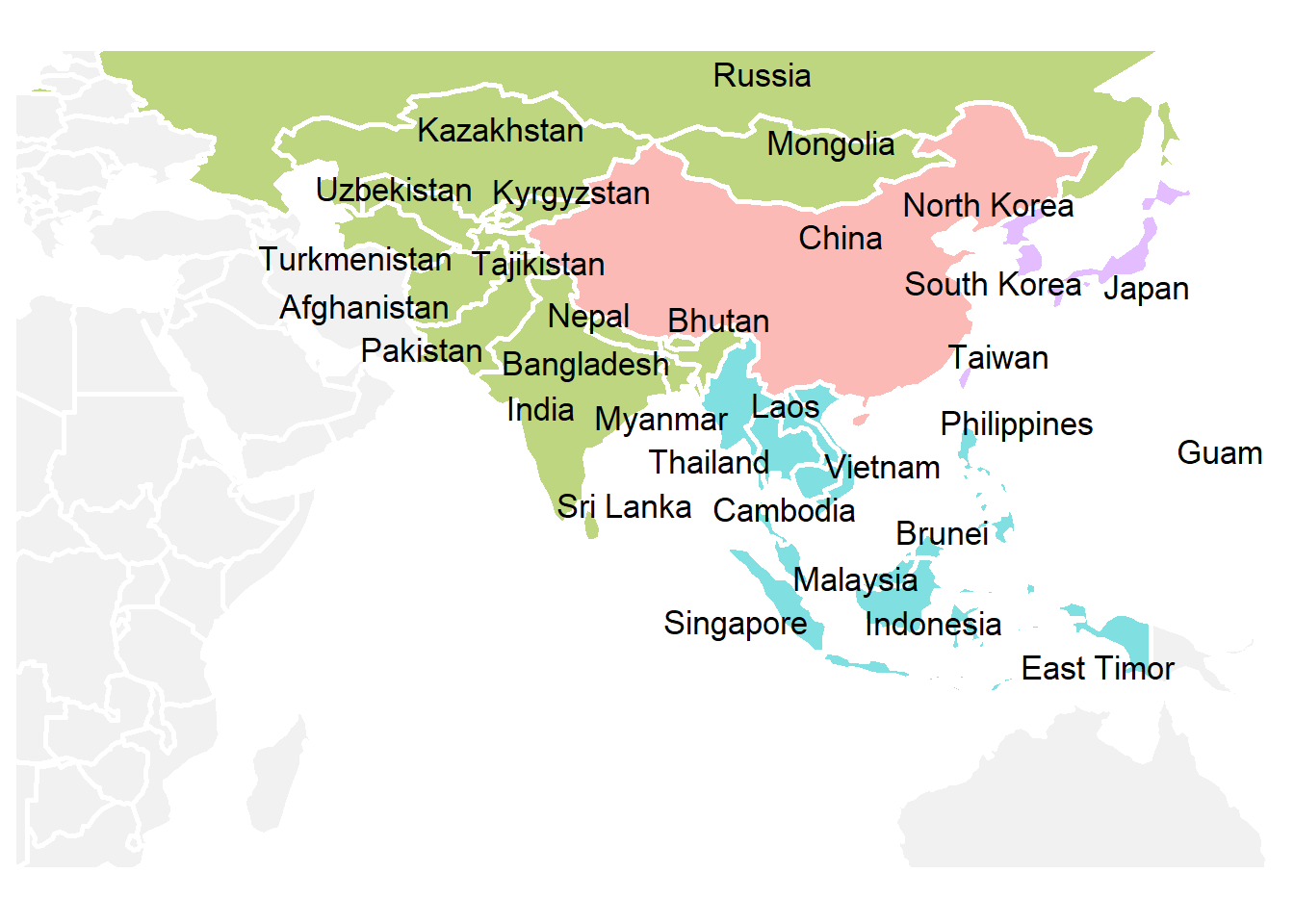

3.2 Map without Raster/Terrain

# Better approach:  Setting dimensions for {r}-snippet according to requirements
# for print would be much better for serialisation and polishing in Illustrator et al.
map <- ggplot() +
 # raster
  # geom_raster(data = relief_land_df, aes(x = x, y = y, alpha = value)) +
  # geom_raster(data = relief_meer_df, aes(x = x, y = y, alpha = value)) +
  # scale_alpha(name = "", range = c(0.4, 0), guide = F) + #  "alpha hack"
  geom_polygon(data = fortify(asia_rest), alpha = 0.5,
               aes(x = long, y = lat, group = group),
               fill = "grey89", color = "white", size = 1) +
  geom_polygon(data = fortify(asia_main), alpha = 0.5,
               aes(x = long, y = lat, group = group, fill = asia_main$category),
               color = "white", size = 1) +
  geom_polygon(data = fortify(Singapore), alpha = 0.5,
               aes(x = long, y = lat, group = group),
               color = "white", fill = "red", size = 1) +
  geom_polygon(data = fortify(Guam), alpha = 0.5,
               aes(x = long, y = lat, group = group),
               color = "white", fill = "red", size = 1) +
  # scale_fill_grey(start = 0.2, end = 0.8) + 
  scale_fill_manual(values = c("#f7f7f7", "#cccccc", "#969696", "#525252")) + 
  # 4-class greya from colorbrewer.org: #f7f7f7 #cccccc #969696 #525252
  coord_equal(ratio = 1, xlim = c(25,149), ylim = c(54.9, -25)) + # cropped
  theme_map() +
  theme(legend.position = "none") +
  geom_text_repel(data = fortify(centroids_df),
                  aes(label = Name, size = 12, x = Long, y = Lat),
                  segment.colour = NA)
plot(map)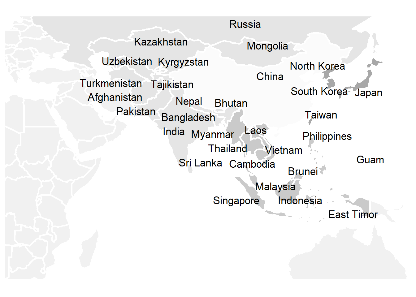

3.3 Map with full Raster (Core & Rest)

Caution: ~3 min rendering time with Intel i7 7500 / 16 GB / SSD

map <- ggplot() +
 # raster
  geom_raster(data = relief_land_df, aes(x = x, y = y, alpha = value)) +
  geom_raster(data = relief_meer_df, aes(x = x, y = y, alpha = value)) +
  scale_alpha(name = "", range = c(0.4, 0), guide = F) + # "alpha hack"
  geom_polygon(data = fortify(asia_rest), alpha = 0.5,
               aes(x = long, y = lat, group = group),
               fill = "grey89", color = "white", size = 1) +
  geom_polygon(data = fortify(asia_main), alpha = 0.5,
               aes(x = long, y = lat, group = group,
                   fill = asia_main$category),
               color = "white", size = 1) +
  geom_polygon(data = fortify(Singapore), alpha = 0.5,
               aes(x = long, y = lat, group = group),
               color = "white", fill = "red", size = 1) +
  geom_polygon(data = fortify(Guam), alpha = 0.5,
               aes(x = long, y = lat, group = group),
               color = "white", fill = "red", size = 1) +
  # scale_fill_grey(start = 0.2, end = 0.8) + 
  scale_fill_manual(values = c("#f7f7f7", "#cccccc", "#969696", "#525252")) + 
  # 4-class grey from colorbrewer.org: #f7f7f7 #cccccc #969696 #525252
  coord_equal(ratio = 1, xlim = c(25,149), ylim = c(54.9, -25)) + # cropped
  theme_map() +
  theme(legend.position = "none") +
  geom_text_repel(data = fortify(centroids_df),
                  aes(label = Name, size = 12, x = Long, y = Lat),
                  segment.colour = NA)
plot(map)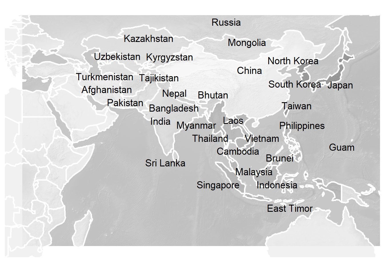

Not perfect, but sufficient for post-processing the output SVG with a vector processing app. One issue I wasn’t able to dissolve, is the different interpretations of the left border set to 25. While the raster definitively is cropped to 25°, the polygons extend beyond that. I’m quite sure that this is because of Kaliningrad, so I guess it should be possible to ID the exclave by “String %in% $var” and exclude it from the dataframe. I might test that later.

Since the map was going to be printed in BW, I decided to provide at least some relieve with regards to the overloaded color scheme. Remember: While ColorBrewer recommends a max of 3 color levels for BW, this map has 4 shades of grey for the 4 core regions, 1 color for water (and borders), and another grey shade for countries which are not part of the core region. Add black for the labels and we end up with 7 colors. So leaving water areas and the rest of the world without relief, while highlighting the core regions by underlying them with a relief kind of works here. Don’t @ me :)

3.4 Final Processing of Output SVG in Affinity Photo / Designer

“Processing the SVG in Affinity”

Basically, I just scaled the SVG to 300 dpi, changed the fonts, moved the labels and slightly readjusted the alpha levels of the regions. That’s it. We’re done here. (PS: We’re not, since someone has to blog about it and maybe even hold it as a lighting talk at a cool workshop)