[R] Joyplots: The (un)joyful Distribution of Grades from German State Exam (Laws)
German Zweites Juristisches Staatsexamen (2nd State Exam in Laws) is said to be tough. Let’s have a look at how hard it really is by visualising the distribution of grades from the Berlin 2017/IV campaign. The written part of the final exam consists of 7 handwritten 5-hour length cases.
Notice that you can score 0-18 points, where a final score of 8 allows you to become a judge and 10 means outstanding…
1 2017/IV Campaign
1.1 Import the Data
Let’s fetch the date from the official page of the Berlin Senate. You’ll get a PDF which you have to destill with the tabulizer package (or by hand) in order to get a CSV. I will follow up with a post on using tabulizer from within RStudio anytime soon.
library(tidyverse)
# Datenquelle: https://www.berlin.de/sen/justiz/juristenausbildung/juristische-pruefungen/artikel.264039.php
data_path <- here::here("static", "data", "/")
noten_raw <- read_csv2(str_c(data_path, "noten_201704.csv")) # nach PDF -> Tabulizer
head(noten_raw) %>% knitr::kable("html", 2)| AZ | Z_I | Z_II | S_I | S_II | OR_I | OR_II | WPF | Dur |
|---|---|---|---|---|---|---|---|---|
| 1014/17 | 8 | 10 | 11 | 15 | 10 | 14 | 9 | 11.00 |
| 1039/17 | 8 | 11 | 13 | 7 | 12 | 11 | 13 | 10.71 |
| 1055/17 | 11 | 11 | 10 | 16 | 6 | 8 | 13 | 10.71 |
| 1097/17 | 15 | 6 | 7 | 16 | 6 | 8 | 13 | 10.14 |
| 0983/17 | 10 | 7 | 8 | 11 | 13 | 10 | 11 | 10.00 |
| 1008/17 | 6 | 14 | 9 | 10 | 11 | 7 | 13 | 10.00 |
1.2 Skim / Preview the Data
The skimr-Package - among others - is great for quickly inspecting what kind of data (variables, data type, NAs etc.) you get.
skimr::skim_to_wide(noten_raw) %>% knitr::kable("html", 2)## Warning: 'skimr::skim_to_wide' is deprecated.
## Use 'skim()' instead.
## See help("Deprecated")| skim_type | skim_variable | n_missing | complete_rate | character.min | character.max | character.empty | character.n_unique | character.whitespace | numeric.mean | numeric.sd | numeric.p0 | numeric.p25 | numeric.p50 | numeric.p75 | numeric.p100 | numeric.hist |
|---|---|---|---|---|---|---|---|---|---|---|---|---|---|---|---|---|
| character | AZ | 0 | 1 | 7 | 7 | 0 | 263 | 0 | NA | NA | NA | NA | NA | NA | NA | NA |
| numeric | Z_I | 0 | 1 | NA | NA | NA | NA | NA | 6.18 | 2.87 | 1.00 | 4.00 | 6.00 | 8.00 | 15 | ▃▇▆▂▁ |
| numeric | Z_II | 0 | 1 | NA | NA | NA | NA | NA | 5.72 | 2.77 | 1.00 | 4.00 | 5.00 | 7.00 | 14 | ▃▇▃▂▁ |
| numeric | S_I | 0 | 1 | NA | NA | NA | NA | NA | 5.90 | 2.91 | 1.00 | 3.00 | 6.00 | 8.00 | 15 | ▆▇▆▃▁ |
| numeric | S_II | 0 | 1 | NA | NA | NA | NA | NA | 5.58 | 2.95 | 0.00 | 3.00 | 5.00 | 7.00 | 16 | ▆▇▅▂▁ |
| numeric | OR_I | 0 | 1 | NA | NA | NA | NA | NA | 5.92 | 2.77 | 2.00 | 4.00 | 5.00 | 8.00 | 14 | ▇▆▆▂▁ |
| numeric | OR_II | 0 | 1 | NA | NA | NA | NA | NA | 5.57 | 2.57 | 1.00 | 4.00 | 5.00 | 7.00 | 14 | ▅▇▃▂▁ |
| numeric | WPF | 0 | 1 | NA | NA | NA | NA | NA | 5.95 | 2.77 | 1.00 | 4.00 | 6.00 | 8.00 | 14 | ▅▇▅▃▁ |
| numeric | Dur | 0 | 1 | NA | NA | NA | NA | NA | 5.83 | 2.01 | 1.42 | 4.28 | 5.57 | 7.28 | 11 | ▂▇▇▅▁ |
(In RStudio / R Markdown the hist column is rendered properly. You get a nice histogram per (numeric) variable. There seems to be an issue with Knitr & UTF-8 encoding on MS Windows systems.)
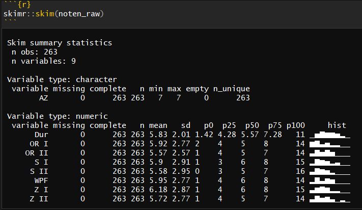
(Screenshot of skimr from RStudio)
1.3 Long -> Short with gather()
Now we need to tidy the data. We first drop the AZ column (Student id) and then “pivot” all the exam subjects into a single column (= variable) named “Fach” (GER for subject).
median_2017 <- median(noten_raw$Dur, na.rm = TRUE)
noten_raw %>%
  select(-AZ) %>%
  gather(key = Fach, value = Punkte) -> noten_long

head(noten_long) %>% knitr::kable("html", 2)| Fach | Punkte |
|---|---|
| Z_I | 8 |
| Z_I | 8 |
| Z_I | 11 |
| Z_I | 15 |
| Z_I | 10 |
| Z_I | 6 |
1.4 2017/IV Joyplot
1.4.1 ggridges-Pkg + colors
We load the ggridges Pkg and the beautiful Viridis color palette
library(ggridges)
library(viridis)
1.4.2 Labels
# Beschriftungen
title_a <- c("2. Juristisches Staatsexamen, GJPA Berlin/Brandenburg")
subtitle_a = paste0("Notenverteilung Kampagne 4/17; n = ",nrow(noten_raw),
                    "; \"Dur\" = durchschnittl. Examensnote\r\nLinien: rot  = \"bestanden (ausreichend)\", blau  = \"vollbefriedigend\",\r\nschwarz  = Median Gesamtnote (",median_2017,")")
caption_a = c("@fubits; Daten: GJPA 2018")
# Plot
noten_long %>%
ggplot() +
geom_density_ridges(aes(x = Punkte, y = Fach, fill = Fach),
rel_min_height = 0.025,
scale = 1.75) +
# Linie: Vollbefriedigend
geom_vline(xintercept = 10, color = "blue", linetype = 4, size = 1) +
# Linie: Bestanden
geom_vline(xintercept = 4, color = "red", linetype = 4, size = 1) +
# Linie: Median Gesamtnote
geom_vline(xintercept = median_2017, color = "black", size = 1) +
labs(title = title_a, subtitle = subtitle_a, caption = caption_a) +
scale_x_continuous(breaks = c(0:18), limits = c(0,18)) +
scale_y_discrete(expand = c(0.01,0.0)) +
scale_fill_viridis(option = "D", name = "Frequency n",
direction = -1, discrete = TRUE) +
# theme(legend.position = "none")
theme_minimal() +
guides(fill = FALSE)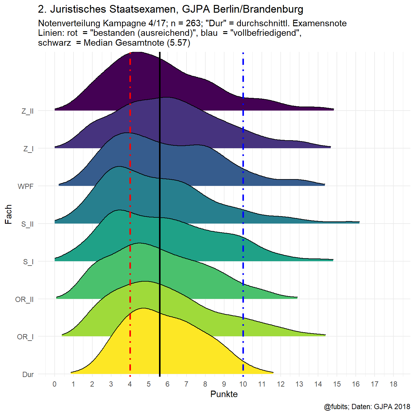
1.5 2017/IV Boxplot
(Dur = overall result / final grade)
noten_long %>%
ggplot() +
  geom_boxplot(aes(x = Fach, y = Punkte, fill = Fach)) +
  scale_y_continuous(breaks = c(0:18), limits = c(0, 18)) +
  scale_fill_viridis(
    option = "C",
    direction = -1, discrete = TRUE
  ) +
  labs(title = title_a, subtitle = subtitle_a, caption = caption_a) +
  # theme(legend.position = "none")
  theme_minimal() +
  guides(fill = FALSE) +
  # Linien zur Orientierung
  geom_hline(yintercept = 10, color = "blue", linetype = 4, size = 1) +
  geom_hline(yintercept = 4, color = "red", linetype = 4, size = 1) +
  geom_hline(yintercept = median_2017, color = "black", size = 1)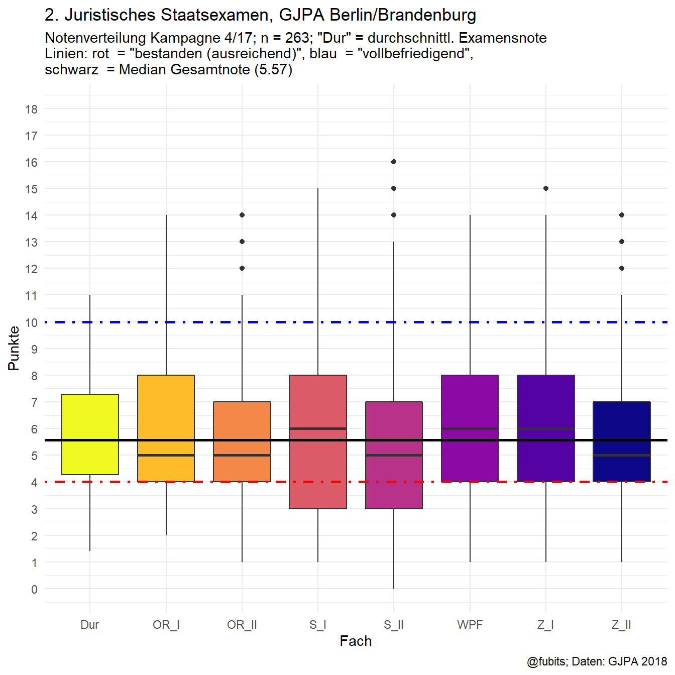
2 Update: 2018/I Campaign
Grades from the 2018/01 campaign just have been released. Let’s plot them for comparison:
# Datenquelle: https://www.berlin.de/sen/justiz/juristenausbildung/juristische-pruefungen/artikel.264039.php
noten_raw_2018 <- read_csv2(str_c(data_path, "noten_201801.csv")) # nach PDF -> Tabulizer
head(noten_raw_2018) %>% knitr::kable("html", 2)| AZ | Z_I | Z_II | S_I | S_II | ÖR_I | ÖR_II | WPF | Dur |
|---|---|---|---|---|---|---|---|---|
| 0874/17 | 7 | 7 | 7 | 4 | 5 | 6 | 10 | 6.57 |
| 0959/17 | 3 | 6 | 2 | 4 | 2 | 4 | 2 | 3.28 |
| 0968/17 | 1 | 3 | 4 | 2 | 3 | 8 | 6 | 3.85 |
| 1001/17 | 3 | 3 | 4 | 2 | 2 | 2 | 2 | 2.57 |
| 1012/17 | 3 | 4 | 2 | 2 | 3 | 2 | 5 | 3.00 |
| 1058/17 | 6 | 10 | 6 | 5 | 7 | 5 | 7 | 6.57 |
skimr::skim_to_wide(noten_raw_2018) %>% knitr::kable("html", 2)## Warning: 'skimr::skim_to_wide' is deprecated.
## Use 'skim()' instead.
## See help("Deprecated")| skim_type | skim_variable | n_missing | complete_rate | character.min | character.max | character.empty | character.n_unique | character.whitespace | numeric.mean | numeric.sd | numeric.p0 | numeric.p25 | numeric.p50 | numeric.p75 | numeric.p100 | numeric.hist |
|---|---|---|---|---|---|---|---|---|---|---|---|---|---|---|---|---|
| character | AZ | 0 | 1 | 7 | 7 | 0 | 277 | 0 | NA | NA | NA | NA | NA | NA | NA | NA |
| numeric | Z_I | 0 | 1 | NA | NA | NA | NA | NA | 5.54 | 2.71 | 1.00 | 3.00 | 5.00 | 7.00 | 14.00 | ▅▇▃▂▁ |
| numeric | Z_II | 0 | 1 | NA | NA | NA | NA | NA | 6.32 | 3.15 | 0.00 | 4.00 | 6.00 | 8.00 | 14.00 | ▂▇▆▃▂ |
| numeric | S_I | 1 | 1 | NA | NA | NA | NA | NA | 5.81 | 2.49 | 1.00 | 4.00 | 6.00 | 7.00 | 14.00 | ▂▇▃▂▁ |
| numeric | S_II | 0 | 1 | NA | NA | NA | NA | NA | 6.12 | 2.82 | 1.00 | 4.00 | 6.00 | 8.00 | 14.00 | ▃▇▅▃▁ |
| numeric | ÖR_I | 0 | 1 | NA | NA | NA | NA | NA | 6.30 | 2.93 | 2.00 | 4.00 | 6.00 | 8.00 | 16.00 | ▇▇▆▂▁ |
| numeric | ÖR_II | 0 | 1 | NA | NA | NA | NA | NA | 5.97 | 2.33 | 1.00 | 4.00 | 6.00 | 8.00 | 13.00 | ▃▆▇▂▁ |
| numeric | WPF | 0 | 1 | NA | NA | NA | NA | NA | 6.00 | 2.91 | 1.00 | 4.00 | 6.00 | 8.00 | 16.00 | ▇▇▆▁▁ |
| numeric | Dur | 1 | 1 | NA | NA | NA | NA | NA | 6.01 | 1.90 | 2.42 | 4.57 | 5.85 | 7.28 | 12.14 | ▅▇▆▂▁ |
median_2018 <- median(noten_raw_2018$Dur, na.rm = TRUE)
noten_raw_2018 %>%
  select(-AZ) %>%
  gather(key = Fach, value = Punkte) -> noten_long_2018

head(noten_long_2018, 1) %>% knitr::kable("html", 2)| Fach | Punkte |
|---|---|
| Z_I | 7 |
title_a <- c("2. Juristisches Staatsexamen, GJPA Berlin/Brandenburg")
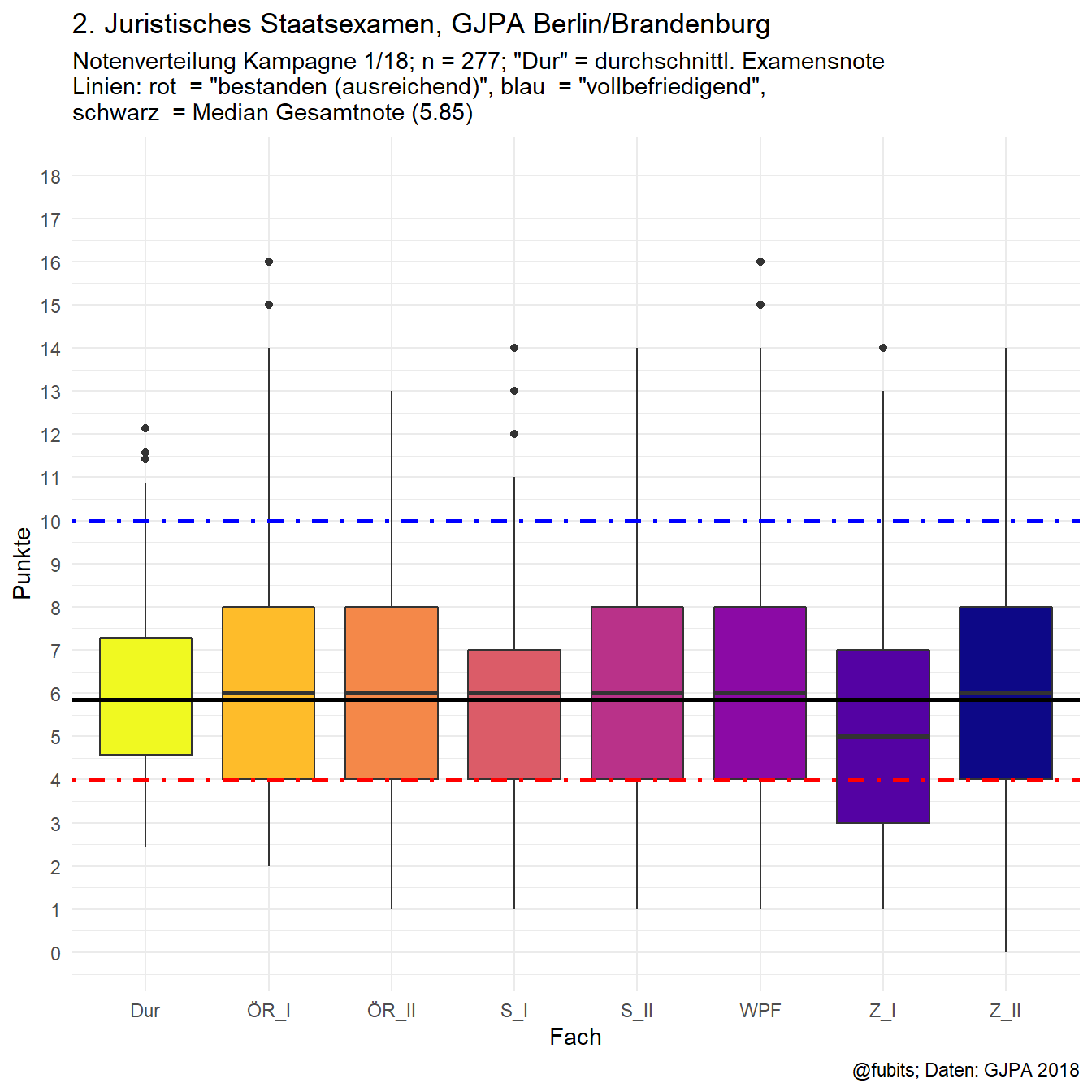
subtitle_a = paste0("Notenverteilung Kampagne 1/18; n = ",nrow(noten_raw_2018),
"; \"Dur\" = durchschnittl. Examensnote\r\nLinien: rot = \"bestanden (ausreichend)\", blau = \"vollbefriedigend\",\r\nschwarz = Median Gesamtnote (",median_2018,")")
caption_a = c("@fubits; Daten: GJPA 2018")2.1 2018/I Joyplot
(Dur = overall result / final grade)
noten_long_2018 %>%
  ggplot() +
  geom_density_ridges(aes(x = Punkte, y = Fach, fill = Fach),
                      rel_min_height = 0.025,
                      scale = 1.75) +
  # Linie: Vollbefriedigend
  geom_vline(xintercept = 10, color = "blue", linetype = 4, size = 1) +
  # Linie: Bestanden
  geom_vline(xintercept = 4, color = "red", linetype = 4, size = 1) +
  # Linie: Median Gesamtnote
  geom_vline(xintercept = median_2018, color = "black", size = 1) +
  labs(title = title_a, subtitle = subtitle_a, caption = caption_a) +
  scale_x_continuous(breaks = c(0:18), limits = c(0,18)) +
  scale_y_discrete(expand = c(0.01,0.0)) +
  scale_fill_viridis(option = "D", name = "Frequency n",
                     direction = -1, discrete = TRUE) +
  # theme(legend.position = "none")
  theme_minimal() +
  guides(fill = FALSE)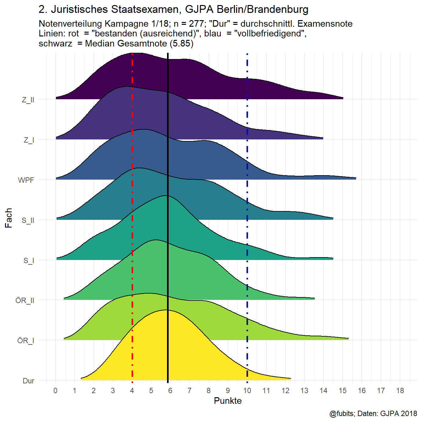
2.2 2018/I Boxplot
noten_long_2018 %>%
ggplot() +
  geom_boxplot(aes(x = Fach, y = Punkte, fill = Fach)) +
  scale_y_continuous(breaks = c(0:18), limits = c(0, 18)) +
  scale_fill_viridis(
    option = "C",
    direction = -1, discrete = TRUE
  ) +
  labs(title = title_a, subtitle = subtitle_a, caption = caption_a) +
  # theme(legend.position = "none")
  theme_minimal() +
  guides(fill = FALSE) +
  # Linien zur Orientierung
  geom_hline(yintercept = 10, color = "blue", linetype = 4, size = 1) +
  geom_hline(yintercept = 4, color = "red", linetype = 4, size = 1) +
  geom_hline(yintercept = median_2018, color = "black", size = 1)